Intracortical smoothing of small-voxel fMRI data can provide increased detection power without spatial resolution losses compared to conventional large-voxel fMRI data

Abstract

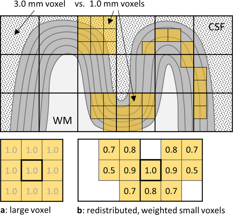
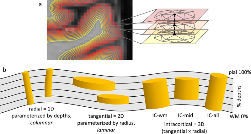
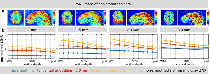
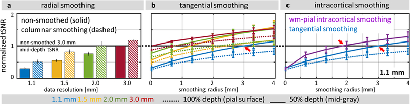
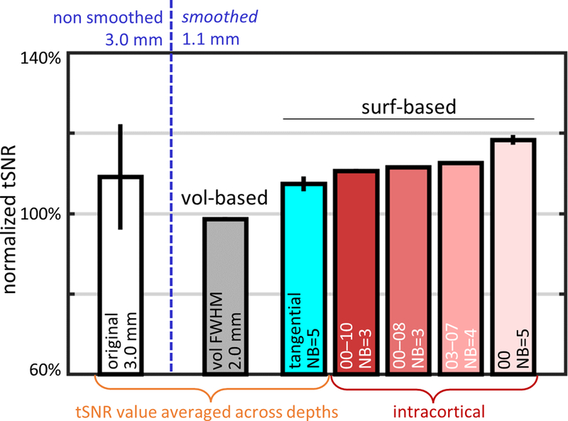
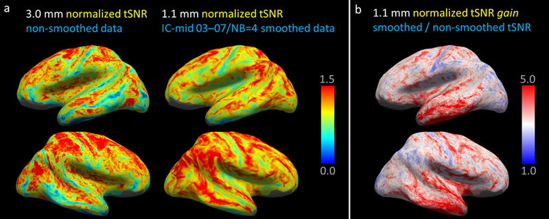
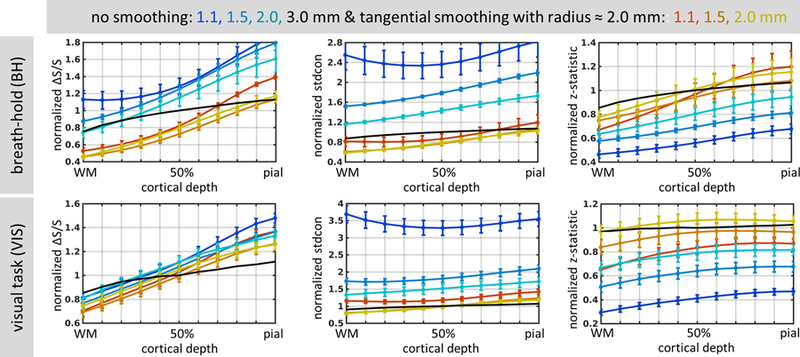
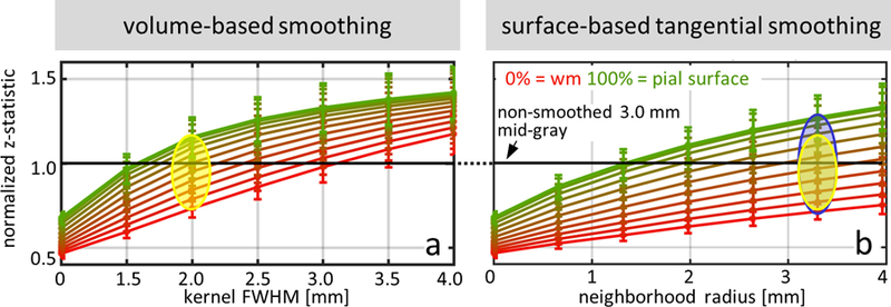
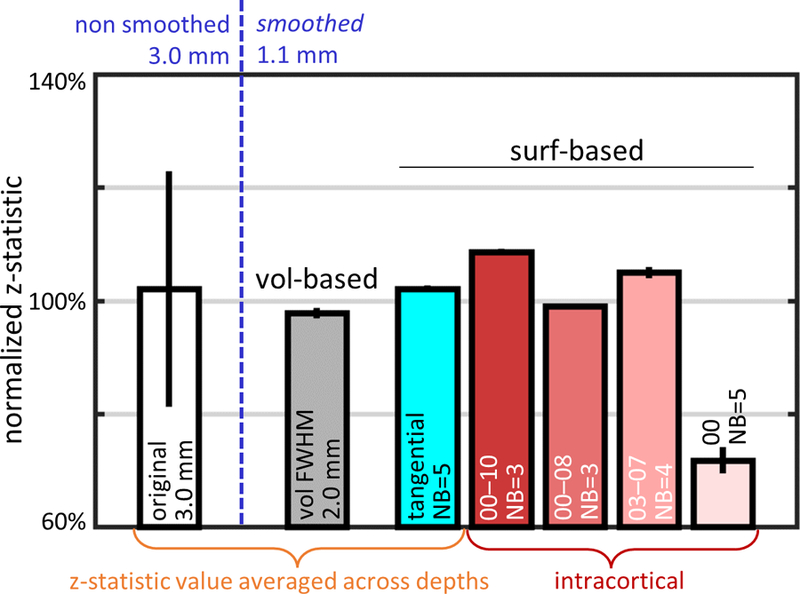
Continued improvement in MRI acquisition technology has made functional MRI (fMRI) with small isotropic voxel sizes down to 1 mm and below more commonly available. Although many conventional fMRI studies seek to investigate regional patterns of cortical activation for which conventional voxel sizes of 3 mm and larger provide sufficient spatial resolution, smaller voxels can help avoid contamination from adjacent white matter (WM) and cerebrospinal fluid (CSF), and thereby increase the specificity of fMRI to signal changes within the gray matter. Unfortunately, temporal signal-to-noise ratio (tSNR), a metric of fMRI sensitivity, is reduced in high-resolution acquisitions, which offsets the benefits of small voxels. Here we introduce a framework that combines small, isotropic fMRI voxels acquired at 7 T field strength with a novel anatomically-informed, surface mesh-navigated spatial smoothing that can provide both higher detection power and higher resolution than conventional voxel sizes. Our smoothing approach uses a family of intracortical surface meshes and allows for kernels of various shapes and sizes, including curved 3D kernels that adapt to and track the cortical folding pattern. Our goal is to restrict smoothing to the cortical gray matter ribbon and avoid noise contamination from CSF and signal dilution from WM via partial volume effects. We found that the intracortical kernel that maximizes tSNR does not maximize percent signal change (ΔS/S), and therefore the kernel configuration that optimizes detection power cannot be determined from tSNR considerations alone. However, several kernel configurations provided a favorable balance between boosting tSNR and ΔS/S, and allowed a 1.1-mm isotropic fMRI acquisition to have higher performance after smoothing (in terms of both detection power and spatial resolution) compared to an unsmoothed 3.0-mm isotropic fMRI acquisition. Overall, the results of this study support the strategy of acquiring voxels smaller than the cortical thickness, even for studies not requiring high spatial resolution, and smoothing them down within the cortical ribbon with a kernel of an appropriate shape to achieve the best performance-thus decoupling the choice of fMRI voxel size from the spatial resolution requirements of the particular study. The improvement of this new intracortical smoothing approach over conventional surface-based smoothing is expected to be modest for conventional resolutions, however the improvement is expected to increase with higher resolutions. This framework can also be applied to anatomically-informed intracortical smoothing of higher-resolution data (e.g. along columns and layers) in studies with prior information about the spatial structure of activation.

Keywords: Columnar fMRI; Cortical depth analysis; High-resolution fMRI; Laminar fMRI; Physiological noise; Spatial smoothing; Surface-based analysis; fMRI analysis.

Fig. 1

A diagram demonstrating the redistribution of small voxels and the weighting of their signals in the process of surface mesh-navigated anatomically-informed smoothing, which allows avoiding CSF and WM influences that commonly affect the signal within large voxels. (a) A large 3×3×3 mm³ voxel effectively smooths (averages) signal from 27 small 1×1×1 mm³ voxels contained within it, using an equal weight of 1.0 for each; here we show the 2D cross-section only, which includes 9 small 1×1×1 mm³ voxels. (b) With smaller voxels, the same volume can be achieved while distributing the voxels such that they are restricted to the cortical ribbon and conform to its shape. Furthermore, the weights can be adapted to provide more flexibility in defining the shape and extent of the kernel.

Fig. 2

(a) A diagram presenting a family of intracortical surface meshes, where the heat scale represents the cortical depth; the mesh topology (i.e., both the numbers of vertices and edges and the connections between the vertices) is the same for all depths, so that a given vertex index in one mesh corresponds to the same vertex index across all the meshes. (b) A schematic illustration of steerable smoothing kernels tracking the cortical GM folds: 1D radial or “columnar”, 2D tangential or “laminar”, and 3D or “intracortical” (IC) extending from WM surface (IC-wm) and from midgray depth (IC-mid), and over all cortical depths (IC-all); columnar smoothing is enacted by an average of the data across the corresponding vertices.

Fig. 3

(a) Example axial slices and sagittal reformats of tSNR maps calculated for all four spatial resolutions (1.1, 1.5, 2.0, 3.0 mm isotropic) of resting-state fMRI data for a representative subject. (Note that different color scales were used across resolutions to better visualize spatial distribution of tSNR.) (b) The effect of tangential smoothing on tSNR values across cortical surfaces, normalized to tSNR of 3.0-mm isotropic resolution non-smoothed data (represented by the black horizontal line), for all four spatial resolutions, averaged across five subjects. Error bars indicate standard error across subjects.

Fig. 4

The effect of radial (columnar), tangential (laminar), and intracortical smoothing on tSNR values of resting-state fMRI data. For comparison, tSNR values were normalized to a reference tSNR of non-smoothed 3.0-mm isotropic resolution data sampled at midgray depth (represented by the black horizontal line), then averaged across five subjects. (a) The results of radial smoothing (dashed bars) are compared with the tSNR of the original data (solid bars) for all four spatial resolutions (1.1, 1.5, 2.0 and 3.0 mm isotropic) and averaged across all cortical depths. (b) The results of tangential smoothing plotted as a function of tangential smoothing radius, for all four spatial resolutions; line colors indicate different spatial resolutions (as in panel a). (c) The results of intracortical smoothing across all depths (IC-all: 00– 10, extending from WM to pial surface) plotted as a function of tangential smoothing radius, for 1.1-mm isotropic resolution data only. For comparison, the tSNR plot of tangential smoothing (blue curve) is reproduced from panel b. In (b) and (c), dashed lines represent data at 100% depth (i.e., at the pial surface), and solid lines represent data at 50% depth (i.e., at the midgray surface); see legend below panel. Red arrows indicate transitions where smoothing of 1.1-mm data produces tSNR that exceeds the tSNR level of the reference non-smoothed 3.0-mm data. Error bars indicate standard error across subjects.

Fig. 5

tSNR values (averaged across 5 subjects) calculated for 1.1-mm isotropic resting-state fMRI data after smoothing with a set of kernels with equivalent smoothing capacities. For comparison, the resulting tSNR was normalized to the reference tSNR of conventional volume-based smoothed data using a 3D kernel with FWHM=2.0 mm sampled at midgray depth. The reference tSNR of the volume-smoothed data, represented by the gray bar, is compared with the tSNR after applying a set of surface-based smoothing kernels with smoothing capacity matched to the FWHM=2.0 mm volume-smoothing kernel: a purely tangential kernel with NB=5 (radius≈3.3 mm, cyan bar) where the resulting tSNR values were averaged across depths, and with intracortical kernels with varying tangential neighborhoods (red-scale bars) including: one extending across all depths (IC-all: 00–10), one extending from the WM to an intermediate depth (IC-wm: 00–08), one centered at midgray depth and extending symmetrically in both directions (IC-mid: 03–07), and one consisting only of the WM surface (IC-wm: 00). Normalized tSNR of non-smoothed 3.0-mm isotropic data was plotted for comparison (white bar). Error bars indicate standard error across subjects.

Fig. 6

Visualization of the spatial distribution of tSNR averaged across subjects using the FreeSurfer CVS avg35 atlas space, shown on the inflated surface representation. (a) Normalized tSNR of the non-smoothed 3.0-mm isotropic resolution data and the 1.1-mm isotropic resolution data after smoothing with surface-based kernel IC-mid 03–07 NB=4. Regional differences in the tSNR maps are seen, however the tSNR of the smoothed 1.1 mm isotropic data is higher than the unsmoothed 3.0-mm isotropic data in nearly every region of the cortical hemispheres. (b) tSNR gain maps showing the tSNR increase, the ratio of 1.1-mm isotropic resolution data smoothed using the kernel from panel (a) by the same non-smoothed 1.1-mm data. For this example acquisition and this example kernel, some brain regions naturally benefit more from smoothing than others.

Fig. 7

Normalized percent signal change (ΔS/S), contrast standard deviation (stdcon), and z-statistic values, averaged across 5 subjects and plotted as a function of cortical depth, for breath-hold (BH, top) and visual task (VIS, bottom), for all spatial resolutions: 1.1, 1.5, 2.0 and 3.0 mm isotropic. Blue-to-cyan lines represent original, non-smoothed data at 1.1, 1.5, and 2.0-mm isotropic resolution, while red-to-yellow lines correspond to data smoothed tangentially with radius of about 2.0 mm (NB=3) at 1.1, 1.5, and 2.0-mm isotropic resolution. Black line represents the values of the non-smoothed 3.0-mm isotropic data for comparison. Error bars indicate standard error across subjects.

Fig. 8

Normalized z-statistic values, averaged across 5 subjects, calculated for 1.1-mm isotropic breath-hold fMRI data, plotted as a function of smoothing kernel size, for all cortical depths (red to green, with red representing data sampled at the WM surface, and green representing data sampled at the pial surface). (a) Conventional 3D volume-based smoothing with various kernel sizes up to 4-mm FWHM. The yellow oval highlights the spread of z-statistic values for a specific kernel size (2-mm FWHM). (b) Proposed 2D tangential surface-based smoothing with radius up to 4 mm. The yellow oval from panel (a) is reproduced here, and is placed at the surface-smoothing radius corresponding to the kernel with smoothing capacity equivalent to the 2.0-mm FWHM 3D volume-smoothing kernel, with the blue oval outlining spread of the z-statistic values across cortical depths (NB=5, radius≈3.3 mm). The blue oval highlights how, at this same smoothing capacity, the surface-based tangential smoothing achieves a broader range of resulting z-statistic values across depths. In both panels the black line represents the reference non-smoothed 3.0-mm isotropic data, and error bars represent standard error across subjects.

Fig. 9

Normalized z-statistic values (averaged across 5 subjects) calculated for 1.1-mm isotropic BH task fMRI data after smoothing with a set of kernels with equivalent smoothing capacities, just as in Fig. 5. The z-statistic values in each subject were first normalized to the z-statistic resulting from conventional volume-based smoothed data using a 3D kernel with FWHM=2.0 mm sampled at midgray depth, then averaged across subjects. The z-statistic of the reference volume-smoothed data, represented by the gray bar, is compared with the z-statistic after applying a set of surface-based smoothing kernels with equivalent smoothing capacity including: a purely tangential kernel with NB=5 (radius≈3.3 mm, cyan bar) where the resulting z-statistic values were averaged across depths, and with intracortical kernels with varying tangential neighborhoods (red-scale bars) including: one extending across all depths (IC-all: 00–10), one extending from the WM to an intermediate depth (IC-wm: 00–08), one centered at midgray depth and extending symmetrically in both directions (IC-mid: 03–07), and one consisting only of the WM surface (IC-wm: 00). Normalized z-statistic of non-smoothed 3.0-mm isotropic data was plotted for comparison (white bar). Error bars indicate standard error across subjects. Unlike the tSNR results shown in Fig. 5, here the normalized z-statistic value of the NB=5 smoothed data at the WM surface is the lowest value of all cases shown.

References

1. Ahveninen J, Chang W-T, Huang S, Keil B, Kopco N, Rossi S, Bonmassar G, Witzel T, Polimeni JR, 2016. Intracortical depth analyses of frequency-sensitive regions of human auditory cortex using 7T fMRI. Neuroimage 143, 116–127. 10.1016/j.neuroimage.2016.09.010 - DOI - PMC - PubMed
1. Andrade A, Kherif F, Mangin JF, Worsley KJ, Paradis AL, Simon O, Dehaene S, Le Bihan D, Poline JB, 2001. Detection of fMRI activation using cortical surface mapping. Hum. Brain Mapp 12, 79–93. - PMC - PubMed
1. Balasubramanian M, Polimeni JR, Schwartz EL, 2010. Near-isometric flattening of brain surfaces. Neuroimage 51, 694–703. 10.1016/j.neuroimage.2010.02.008 - DOI - PMC - PubMed
1. Barth M, Breuer F, Koopmans PJ, Norris DG, Poser BA, 2016. Simultaneous multislice (SMS) imaging techniques. Magn. Reson. Med 75, 63–81. 10.1002/mrm.25897 - DOI - PMC - PubMed
1. Bazin PL, Weiss M, Dinse J, Schäfer A, Trampel R, Turner R, 2014. A computational framework for ultra-high resolution cortical segmentation at 7 Tesla. Neuroimage 93, 201–209. 10.1016/j.neuroimage.2013.03.077 - DOI - PubMed
Publication types