A scalable discrete-time survival model for neural networks

Abstract

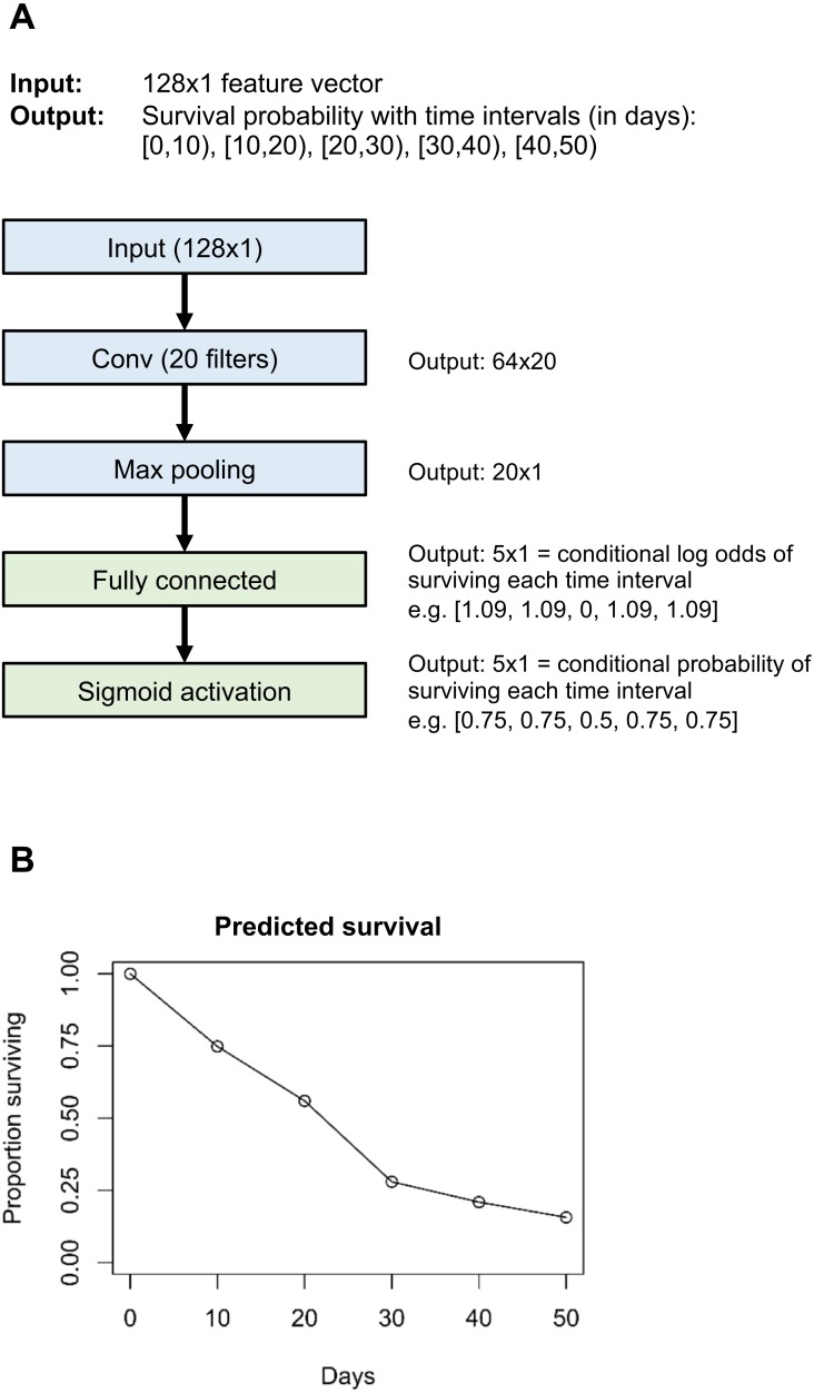
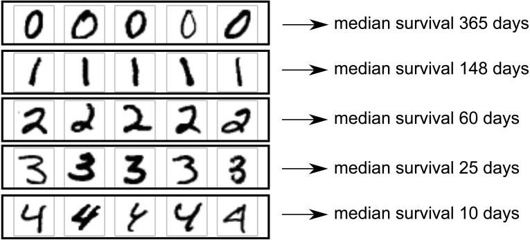
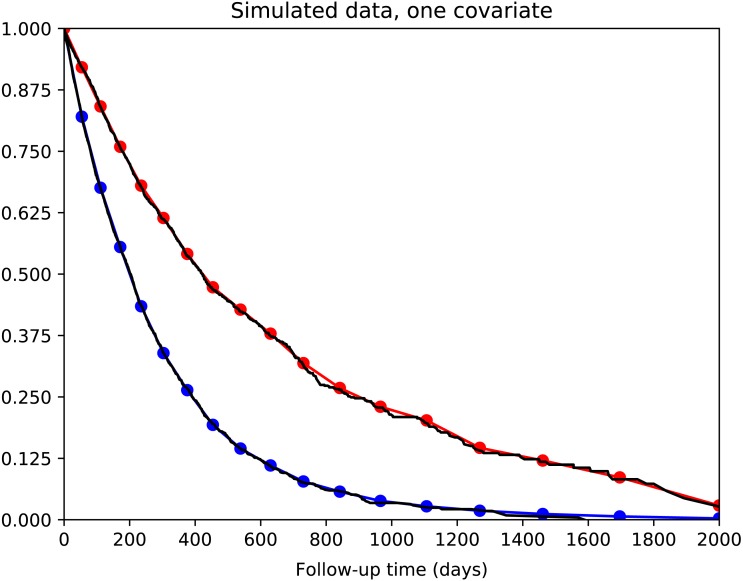
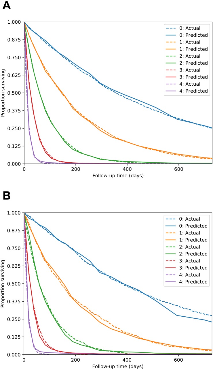
There is currently great interest in applying neural networks to prediction tasks in medicine. It is important for predictive models to be able to use survival data, where each patient has a known follow-up time and event/censoring indicator. This avoids information loss when training the model and enables generation of predicted survival curves. In this paper, we describe a discrete-time survival model that is designed to be used with neural networks, which we refer to as Nnet-survival. The model is trained with the maximum likelihood method using mini-batch stochastic gradient descent (SGD). The use of SGD enables rapid convergence and application to large datasets that do not fit in memory. The model is flexible, so that the baseline hazard rate and the effect of the input data on hazard probability can vary with follow-up time. It has been implemented in the Keras deep learning framework, and source code for the model and several examples is available online. We demonstrate the performance of the model on both simulated and real data and compare it to existing models Cox-nnet and Deepsurv.

Keywords: Machine learning; Neural networks; Survival analysis.

Figure 1. Example neural network architecture (A) and output for one individual (B).

Layers in blue are unique to the example neural network; layers in green are common to all neural networks that use the “flexible” version of our survival model.

Figure 2. MNIST dataset construction.

Images of handwritten digits 0–4 were used as predictor of survival time (one image per patient). Actual survival time was generated from an exponential distribution with scale depending on the digit. Lower digits have longer median survival.

Figure 3. Simple survival model with one predictor variable.

5,000 simulated patients with exponential survival distribution. Half of patients have predictor variable value of 0 with median survival of 200 days; the other half have value of 1 with median survival of 400 days. Actual survival for the two groups is shown in black (Kaplan–Meier curves). The average model predictions for the two groups are shown in blue and red, respectively. Model predictions correspond well to actual survival.

Figure 4. MNIST dataset calibration plots for training set (A) and test set (B).

Images of handwritten digits 0–4 were used as predictor of survival time. Lower digits have longer median survival. For each digit, actual survival curve plotted with dotted line and mean model-predicted survival plotted with solid line.

Figure 5. Example of violation of proportional hazards assumption in SUPPORT study dataset.

For the “ca” variable, patients with metastatic cancer have a similar risk of early death as other patients, but a higher risk of late death, as evidenced by non-parallel lines on this plot of log(-log survival) over time.

Figure 6. Calibration of four survival models on SUPPORT study test set.

For each model, for each of three follow-up times, patients were grouped by deciles of predicted survival probability. Then, for each decile, mean actual survival (Kaplan–Meier method) was plotted against mean predicted survival. A perfectly calibrated model would have all points on the identity line (dashed). Follow-up times: (A) 6 months; (B) 1 year; (C) 3 years.

Figure 7. Running time of the three neural network models on SUPPORT study dataset.

Each point represents the average of three runs. Cox-nnet ran out of memory for sample sizes of 100,000 and higher.

References

1. Avati A, Jung K, Harman S, Downing L, Ng A, Shah NH. Improving palliative care with deep learning. 20171711.06402 - PMC - PubMed
1. Bottou L. Stochastic gradient learning in neural networks. Proceedings of Neuro-Nimes. 1991;91(8):687–706.
1. Breslow N. Covariance analysis of censored survival data. Biometrics. 1974;30:89–99. - PubMed
1. Breslow N, Crowley J. A large sample study of the life table and product limit estimates under random censorship. The Annals of Statistics. 1974;2(3):437–453. doi: 10.1214/aos/1176342705. - DOI
1. Brown SF, Branford AJ, Moran W. On the use of artificial neural networks for the analysis of survival data. IEEE Transactions on Neural Networks. 1997;8(5):1071–1077. doi: 10.1109/72.623209. - DOI - PubMed
LinkOut - more resources