Towards a sampling design for characterizing habitat-specific benthic biodiversity related to oxygen flux dynamics using Aquatic Eddy Covariance

Abstract

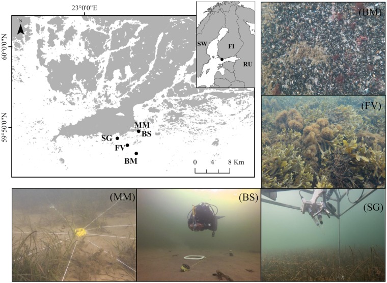
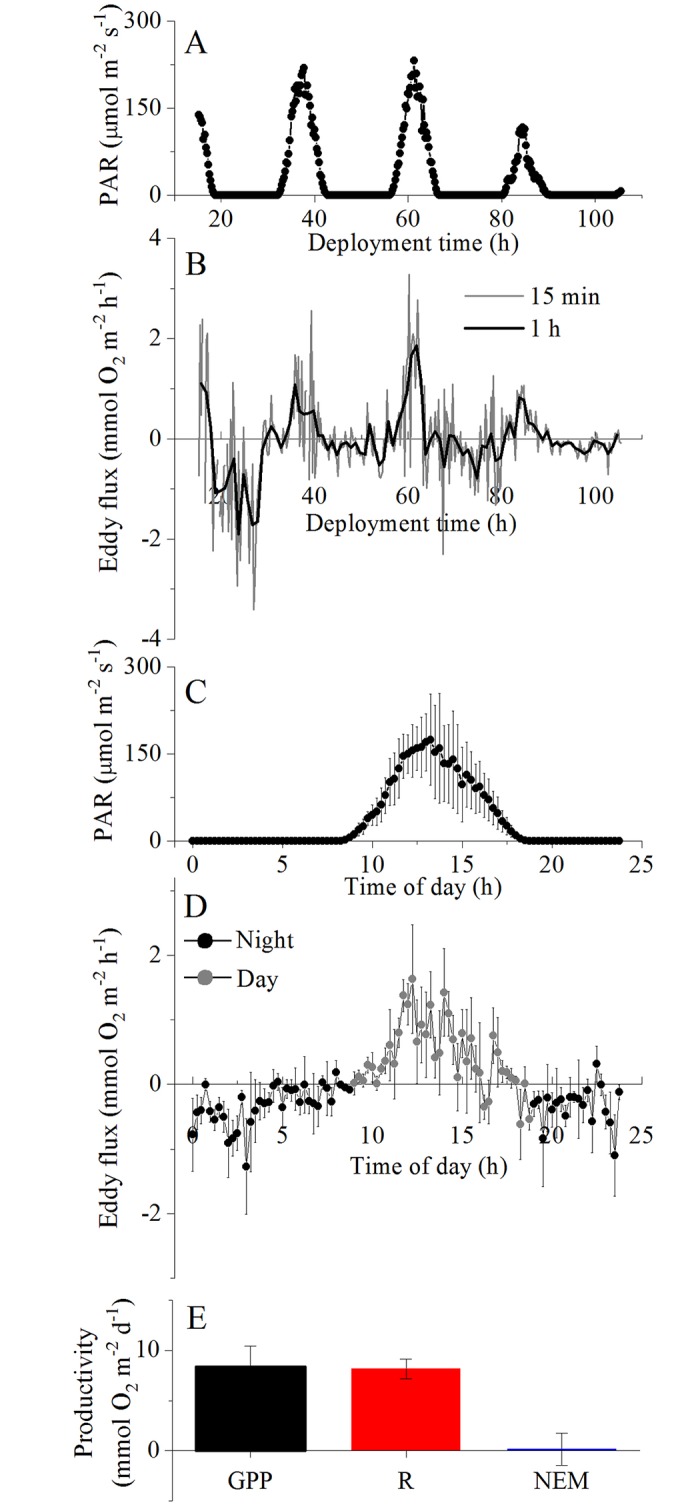
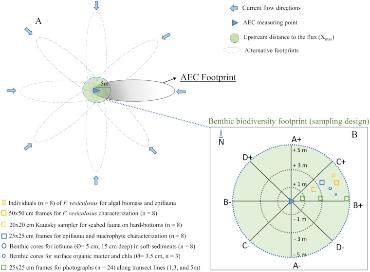
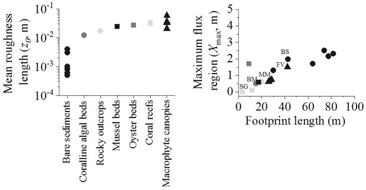
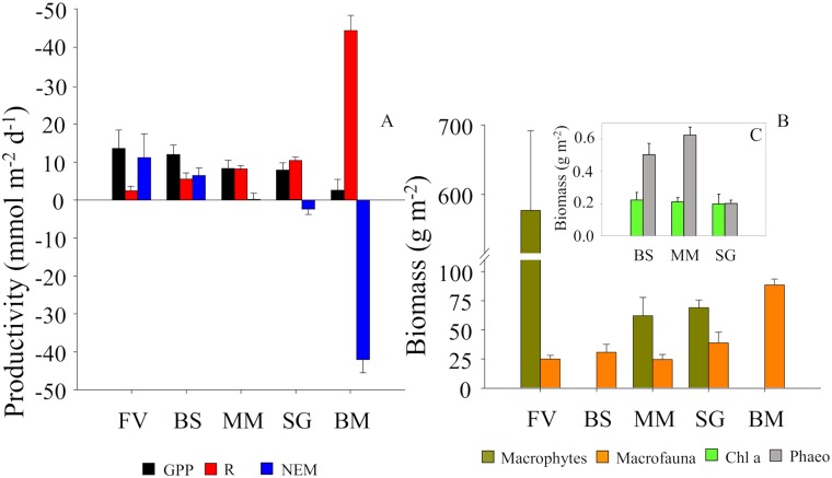
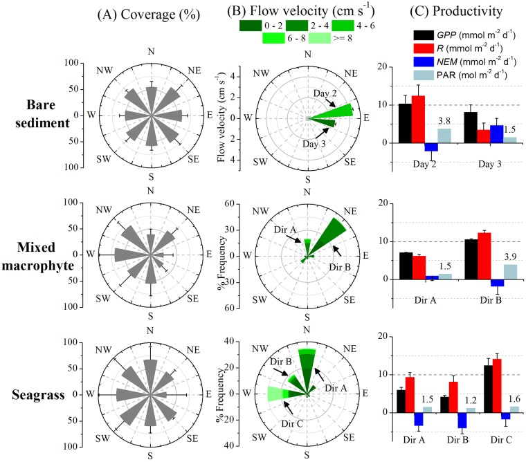
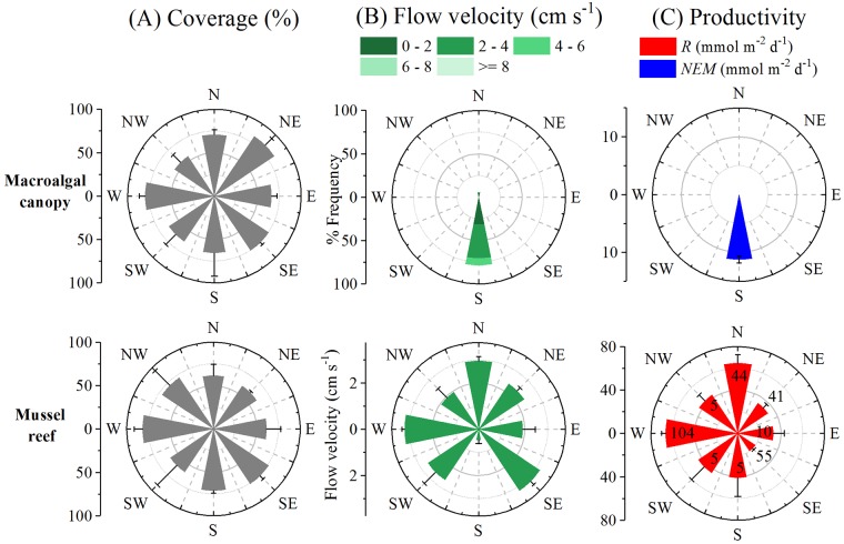
The Aquatic Eddy Covariance (AEC) technique has emerged as an important method to quantify in situ seafloor metabolism over large areas of heterogeneous benthic communities, enabling cross-habitat comparisons of seafloor productivity. However, the lack of a corresponding sampling protocol to perform biodiversity comparisons across habitats is impeding a full assessment of marine ecosystem metabolism. Here, we study a range of coastal benthic habitats, from rocky-bed communities defined by either perennial macroalgae or blue mussel beds to soft-sediment communities comprised of either seagrass, patches of different macrophyte species or bare sand. We estimated that the maximum contribution to the AEC metabolic flux can be found for a seafloor area of approximately 80 m2 with a 5 meter upstream distance of the instrument across all the habitats. We conducted a sampling approach to characterize and quantify the dominant features of biodiversity (i.e., community biomass) within the main seafloor area of maximum metabolic contribution (i.e., gross primary production and community respiration) measured by the AEC. We documented a high biomass contribution of the macroalgal Fucus vesiculosus, the seagrass Zostera marina and the macroinvertebrate Mytilus edulis to the net ecosystem metabolism of the habitats. We also documented a significant role of the bare sediments for primary productivity compared to vegetated canopies of the soft sediments. The AEC also provided insight into dynamic short-term drivers of productivity such as PAR availability and water flow velocity for the productivity estimate. We regard this study as an important step forward, setting a framework for upcoming research focusing on linking biodiversity metrics and AEC flux measurements across habitats.

Fig 1. Map of the Baltic Sea archipelago (SW Finland) showing the locations of the habitats.

Mixed macrophyte (MM) and bare sand (BS) habitats, exposed seagrass meadow (SG), littoral bladder-wrack belt (FV), and blue mussel reef (BM). A selection of photographs showing the biodiversity sampling area at the MM and BS, the AEC deployed at the SG, and a closer look to the Fucus vesiculosus and blue mussels at the BM and FV rocky beds, respectively.

Fig 2. Example of eddy covariance data treatment for calculating daily seafloor productivity rates from the MM site.

The collected datasets for PAR (15 min, A) and the eddy fluxes (15 min, B) were bin-averaged by the hour of day to produce a single 24 h time series for PAR (C, mean ± SD, n = 3) and eddy flux (D, mean ± SE, n = 3). The eddy flux time series was separated into day-time and night-time fluxes to compute daily rates of seafloor gross primary productivity (GPP), respiration (R), and net ecosystem metabolism (NEM) (E, in mmol O₂ m^-2 d^-1, see Methods).

Fig 3. Schematic illustration of the AEC footprint and biodiversity sampling area.

(A) Diagram from above showing the AEC footprint areas determined by different flow directions. The length, width and total area of the AEC footprints for all the habitats are shown in Table 1. The circular biodiversity footprint (80 m², r = 5 m) was superimposed to the AEC footprint ensuring that the maximum flux contribution measured in all the habitats (X_max = 5 m) was covered. The grey scale shows a theoretical gradient of the benthic contribution to the flux registered within the footprint area (darker grey implies higher contribution closer to the device). (B) Illustration of the biodiversity footprint area displaying 8 equal wedge-sections for community characterization. Quantitative random samples (n = 8, one replicate sample per each of the 8 wedge-sections) of the main benthic organisms (v macrofauna, macrophytes and macroalgae) were collected (see Methods).

Fig 4. Estimated characteristics of the AEC footprint.

Mean roughness length (z₀) and estimated footprint length versus region of maximum flux contribution (X_max) for various coastal benthic habitats (Bare sediments: [,,,, this study]; Coralline algal bed: [27]; Rocky outcrop: [31]; Mussel bed: [this study]; Oyster bed: [20]; Coral reef: [33]; Vegetated canopy: [,, this study]). The estimated footprint values (length vs X_max) for the study sites were allocated (i.e., BS: bare sand; MM: mixed macrophyte; SG: seagrass meadow; FV: bladder-wrack belt; BM: blue mussel).

Fig 5. Mean (+SE) ecosystem metabolism and benthic biodiversity biomass.

(A) Ecosystem metabolism (GPP: gross primary production, R: community respiration, NEM: net ecosystem metabolism), (B) benthic biomass (dry weight) of macrophytes (Z. marina and Fucus vesiculosus) and macrofauna (total average), and (C) benthic biomass (dry weight) of chlorophyll a (Chl a) and phaeopigments (Phaeo) from all the habitats (FV: bladder-wrack bed, BS: bare sand, MM: mixed macrophyte, SG: seagrass meadow, BM: blue mussel reef). Different letters represent significant differences (p < 0.05) for the main metrics.

Fig 6. Windrose plots (mean ± SD) for the soft-sediment sites.

(A) Coverage (ArcMap, see section 2.7.) of benthic microalgae (i.e., chlorophyll a), macrophytes, and seagrass, (B) directional flow velocity distribution, and (C) daily seafloor productivity rates for different days or different directions (daily integrated PAR values are indicated).

Fig 7. Windrose plots (mean ± SD) for rocky substrates.

(A) Coverage (ArcMap, see section 2.7.) of macroalgae and mussels, (B) directional flow velocity distribution, and (C) corresponding seafloor productivity rates, indicating the number of 15 min fluxes.

References

1. Snelgrove PVR, Thrush SF, Wall DH, Norkko A. Real world biodiversity-ecosystem functioning: a seafloor perspective. 2014; Trends Ecol Evol. 29:398–405. 10.1016/j.tree.2014.05.002 - DOI - PubMed
1. Lohrer AM, Thrush SF, Gibbs MM. Bioturbators enhance ecosystem function through complex biogeochemical interactions. 2004; Nature 431:1092–1095. 10.1038/nature03042 - DOI - PubMed
1. Lohrer AM, Thrush SF, Hewitt JE, Kraan C. The up-scaling of ecosystem functions in a heterogeneous world. 2015; Sci Rep. 5:10349 10.1038/srep10349 - DOI - PMC - PubMed
1. Glud RN. Oxygen dynamics of marine sediments. 2008; Mar Biol Res. 4:243–289.
1. Duffy EJ. Why biodiversity is important to the functioning of real-world ecosystems. 2009; Front Ecol Environ. 7(8):437–444.
Publication types