Ocean colour signature of climate change

Abstract

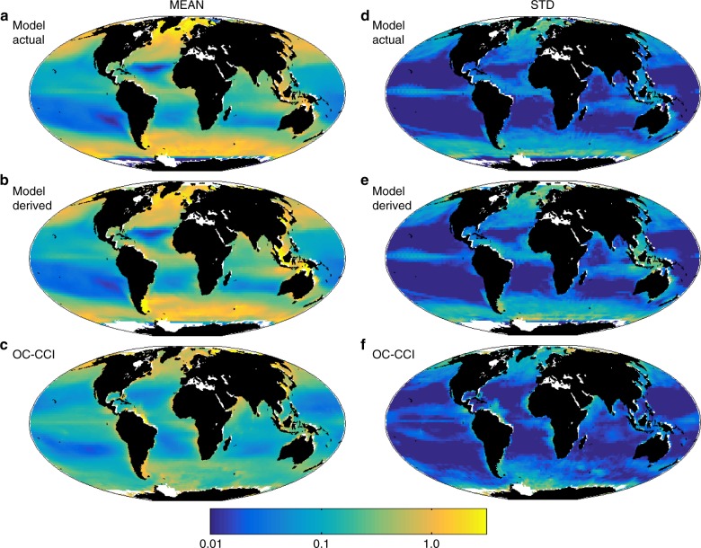
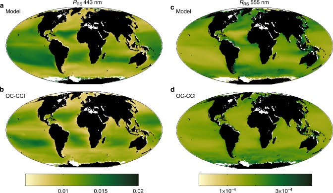
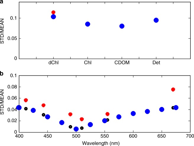
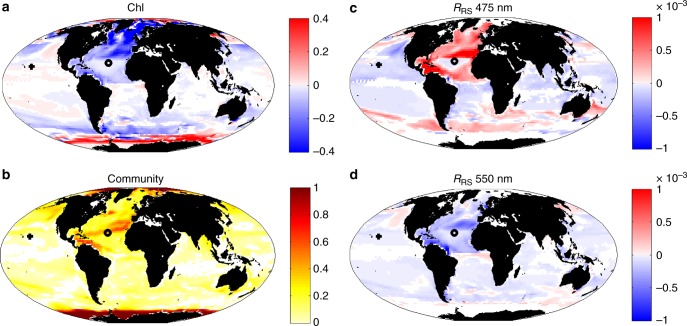
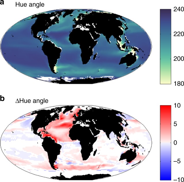
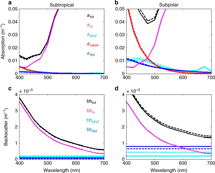
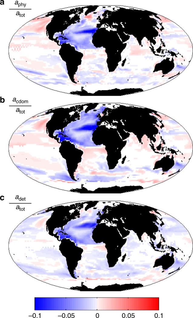
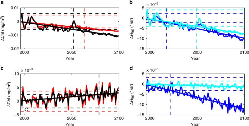
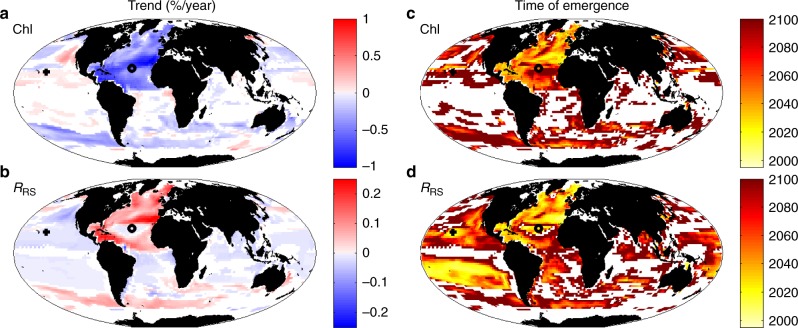
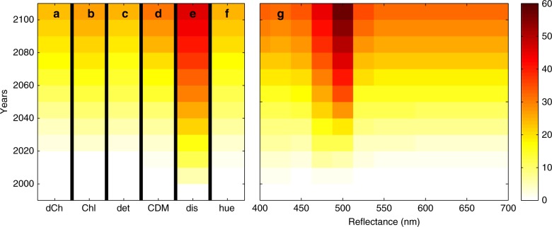
Monitoring changes in marine phytoplankton is important as they form the foundation of the marine food web and are crucial in the carbon cycle. Often Chlorophyll-a (Chl-a) is used to track changes in phytoplankton, since there are global, regular satellite-derived estimates. However, satellite sensors do not measure Chl-a directly. Instead, Chl-a is estimated from remote sensing reflectance (R_RS): the ratio of upwelling radiance to the downwelling irradiance at the ocean's surface. Using a model, we show that R_RS in the blue-green spectrum is likely to have a stronger and earlier climate-change-driven signal than Chl-a. This is because R_RS has lower natural variability and integrates not only changes to in-water Chl-a, but also alterations in other optically important constituents. Phytoplankton community structure, which strongly affects ocean optics, is likely to show one of the clearest and most rapid signatures of changes to the base of the marine ecosystem.

Fig. 1

Current day Chl-a and its interannual variability. Composite mean Chl-a (mg Chl m⁻³) for 1998–2015: a model actual; b model satellite-like derived (using an algorithm and the model R_RS,); c Ocean Colour Climate Change Initiative project (OC-CCI, v2) satellite derived. Interannual variability defined as the standard deviation of the annual mean composites (1998–2015): d model actual; e model satellite-like derived; f OC-CCI, v2 satellite derived. White areas are regions where model resolution is too coarse to capture the smaller seas, or where there is persistent ice cover. Statistical comparison of derived model and OC-CCI product are provided in Supplementary Figs. 1–3. Model actual Chl-a is the sum of the dynamic Chl-a for each phytoplankton type that is explicitly resolved in the model. It is equivalent to the Chl-a that would be measured in situ. This is distinct to satellite-derived Chl-a which is calculated via an algorithm derived from the reflected light measured by ocean colour satellite instruments

Fig. 2

Remotely sensed reflectance. Current day composite (1998–2015) for a model R_RS interpolated to 443 nm, b observed R_RS at 443 nm, c model R_RS interpolated to 555 nm, and d observed R_RS at 555 nm. Units are sr⁻¹. Observed fields are from the Ocean Colour Climate Change Initiative (OC-CCI) project. White areas are regions where model resolution is too coarse to capture the smaller seas or regions of constant ice cover. Statistics of comparison of model and all six observed wavebands are provided in Supplementary Figs. 1, 2

Fig. 3

Relative magnitude of interannual variability. Global median of the ratio of the annual composite temporal standard deviation to the 18 year mean composite for a satellite derived Chl-a (dChl), actual Chl-a (Chl), detrital matter (det) and CDOM; and for b remotely sensed reflectance. Blue indicates model output, red for OC-CCI products, and black for the model interpolated to the OC-CCI wavebands. The OC-CCI reflectances are at 412, 443, 490, 510, 555, 670 nm. See Supplementary Fig. 4 for spatial patterns of relative magnitude or both model of OC-CCI products

Fig. 4

Change between current day and end of the 21st century. a Difference in model actual Chl-a (mg Chl m⁻³) between 2085–2100 mean and the current day (1998–2015) mean. b Change to phytoplankton community structure as defined from Bray–Curtis dissimilarity index for community structure averaged over 2085–2100 versus the present day community (1998–2015). 0 indicates no change, 1 indicates a completely new community. Difference in model R_RS 2085–2100 mean and the current day (1998–2015) mean for c 475 nm (blue) and d 550 nm (green). In all panels only areas with statistically significant differences between the two periods (p < 0.05) are shown. In addition, in c and d we only show regions which were ice free for most of the year (i.e. open ocean where R_RS was calculated) in the current day. The symbols (+,o) indicate two locations highlighted in Fig. 8

Fig. 5

Hue angle. a Mean for 1998–2015, b difference in model 2085–2100 mean and the current day (1998–2015). In b only areas with a statistically significant differences between the two periods (p < 0.05) and which were ice free for most of the year (i.e. open ocean where R_RS was calculated) in the current day are shown

Fig. 6

Absorption and backscatter. Components of total absorption (a, b) and backscattering (c, d) for two locations: middle of the oligotrophic subtropical gyre (circle in Fig. 4) (a, c) and the productive subpolar gyre in the North Atlantic (b, d). Units are m⁻¹. Solid lines are for current day (15 year mean) and dashed lines are for the mean of the last 15 years of the 21st century. Black is for total, purple for water, red for coloured dissolved organic matter (CDOM), light blue for phytoplankton, and dark blue for detrital particles

Fig. 7

Change in contribution of optically important constituents. Change between 2085–2100 and 1998–2015 of a a_phy/a_tot; b a_cdom/a_tot; c a_det/a_tot at 475 nm. Absorption is indicated by a: a_tot refers to total absorption, a_phy to the phytoplankton component of absorption, a_cdom to the dissolved organic matter component, and a_det to the detrital particle component. Only regions with statistically significant differences (p < 0.05) between the two sample periods are shown. In addition, we only show regions that were ice free for most of the year

Fig. 8

Time series of changes in two locations. a, b are in the North Atlantic, indicated by circle in Fig. 4. c, d are in North Pacific, indicated by cross in Fig. 4. a and c show the changes in model actual Chl-a (black) and model Chl-a product derived from reflectance ratio (red); b, d show changes in R_RS for 475 nm (dark blue) and 550 nm (light blue). Straight solid lines indicate the linear trend using generalized least squares (GLS), the dashed horizontal lines indicate plus and minus two standard deviations (STD) of the interannual variability from 1998 to 2015, and the vertical dashed line shows the time of emergence (trend > twice the STD)

Fig. 9

Trends and time of emergence. Model linear trend (%/year) for a actual Chl-a, and b remotely sensed reflectance at 475 nm; and time of emergence of trend for c Chl-a, and d R_RS at 475 m. A generalized least squares (GLS) fit was used to quantify the trends. Only regions with statistically significant (p < 0.05) trends over the 21st century and that were largely ice-free in the current day (as model R_RS are only valid for such regions) are shown. The symbols (+,o) indicate two locations highlighted in Fig. 8

Fig. 10

Percent ocean area with significant trend. The amount of open ocean area that has statistically significant trend (p < 0.05) since 1995 with 5-year increments. a Satellite-like derived Chl-a is the blue/green reflectance ratio Chl-a product calculated with an OC4-like algorithm, b actual Chl-a is the sum of the 8 dynamically changing phytoplankton which contribute to total Chl-a (as might be measured in situ); c detritus is the non-living particulate organic pool, d CDOM is the coloured dissolved organic matter, e dis refers to Bray–Curtis Dissimilarity index, and is a measure of the changes to the phytoplankton community structure; f hue refers to the hue angle, α, a metric of true colour; g the remotely sensed reflectance in the visible spectrum, in 13 wavebands

References

1. IOCCG. Atmospheric Correction for Remotely-Sensed Ocean-Colour Products. (ed. Wang, M.), Reports of the International Ocean-Colour Coordinating Group, No.10 (IOCCG, Dartmouth, 2010) .
1. O’Reilly, J. E. et al. SeaWiFS Postlaunch Calibration and Validation Analyses, Part 3. NASA Tech. Memo. 2000-206892, Vol. 11 (eds. Hooker, S. B. & Firestone, E.R.) (NASA Goddard Space Flight, 2001).
1. Maritorena S, Siegel DA, Peterson A. Optimization of a semi-analytical ocean color model for global scale applications. Appl. Opt. 2002;41:2705–2714. doi: 10.1364/AO.41.002705. - DOI - PubMed
1. Werdell PJ, et al. An overview of approaches and challenges for retrieving marine inherent optical properties from ocean color remote sensing. Progress. Oceanogr. 2018;160:186–212. doi: 10.1016/j.pocean.2018.01.001. - DOI - PMC - PubMed
1. Antoine D, Morel A, Gordon HR, Banzon VF, Evans RH. Bridging ocean color observations of the 1980s and 2000s in search of long-term trends. J. Geophys. Res. 2005;110:C06009. doi: 10.1029/2004JC002620. - DOI
Publication types