A Random Forests Quantile Classifier for Class Imbalanced Data

Abstract

Extending previous work on quantile classifiers (q-classifiers) we propose the q*-classifier for the class imbalance problem. The classifier assigns a sample to the minority class if the minority class conditional probability exceeds 0 < q* < 1, where q* equals the unconditional probability of observing a minority class sample. The motivation for q*-classification stems from a density-based approach and leads to the useful property that the q*-classifier maximizes the sum of the true positive and true negative rates. Moreover, because the procedure can be equivalently expressed as a cost-weighted Bayes classifier, it also minimizes weighted risk. Because of this dual optimization, the q*-classifier can achieve near zero risk in imbalance problems, while simultaneously optimizing true positive and true negative rates. We use random forests to apply q*-classification. This new method which we call RFQ is shown to outperform or is competitive with existing techniques with respect to tt-mean performance and variable selection. Extensions to the multiclass imbalanced setting are also considered.

Keywords: Class Imbalance; Minority Class; Random Forests; Response-based Sampling; Weighted Bayes Classifier.

Figure 1:

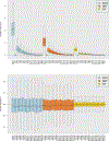
Summary of 143 benchmark imbalanced data sets. Top figures display dimension of feature space d, sample size N, and imbalance ratio IR. Bottom figure displays d versus N with symbol size displaying value of IR. This identifies several interesting data sets with large IR values, with some of these having larger d.

Figure 2:

G-mean from random forests q-classification using various q for thresholding $\left(\text{including}\hspace{0.17em}q=\widehat{\pi }\right)$ for 8 different bench-mark data sets. Notice that the maximum value is near $\widehat{\pi }$ in all instances.

Figure 3:

G-mean performance of different classifiers across 143 benchmark imbalanced data sets. (BRF=Balanced Random Forests; RF=Random Forests; RFQ = Random Forests q*-classifier).

Figure 4:

A closer look at difference in G-mean performance of RFQ and BRF for benchmark data sets. Vertical axis plots difference in G-mean as a function of % rare minority class examples, feature dimension d, and imbalance ratio IR. There is an increasing trend upwards (thus favoring RFQ) as % rare minority class examples increases with increasing d and increasing IR.

Figure 5:

Variable importance (VIMP) for RFQ, BRF and RF from 1000 runs using simulated imbalanced data. There are 2 factors, 15 linear variables, 3 non-linear variables, and 20 noise variables (no signal). Top panel displays signal variables, bottom panel are noisy variables.

Figure 6:

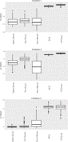
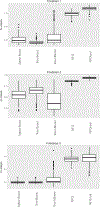
G-mean performance of boosting classifiers versus RFQ for Friedman low dimensional simulations. (Spline Boost, Tree Boost are boosted splines and boosted trees using binomial loss; Tree HBoost are boosted trees with Huber loss; RFQvsel is RFQ with variable selection filtering).

Figure 7:

G-mean performance of boosting classifiers versus RFQ for Friedman high dimensional simulations. (Spline Boost, Tree Boost are boosted splines and boosted trees using binomial loss; Tree HBoost are boosted trees with Huber loss; RFQvsel is RFQ with variable selection filtering).

Figure 8:

Computational times for RFQ and BRF for Friedman 1 simulation for different sample sizes N and feature dimension d. Top plot is relative CPU time for RFQ versus BRF. Bottom plot is log-relative CPU time.

References

1. Breiman L, Random forests, Machine Learning 45 (1) (2001) 5–32.
1. Verikas A, Gelzinis A, Bacauskiene M, Mining data with random forests: A survey and results of new tests, Pattern Recognition 44 (2) (2011) 330–349.
1. Biau G, Scornet E, A random forest guided tour, Test 25 (2) (2016) 197–227.
1. Breiman L, Manual on Setting up, Using, and Understanding Random Forests V3 1, 2002.
1. Ishwaran H, Variable importance in binary regression trees and forests, Electronic Journal of Statis-tics 1 (2007) 519–537.
LinkOut - more resources