Assessing the practical differences between model selection methods in inferences about choice response time tasks

Abstract

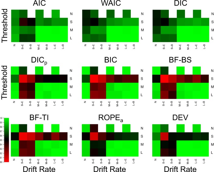
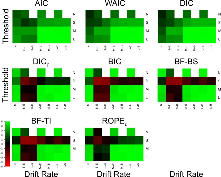
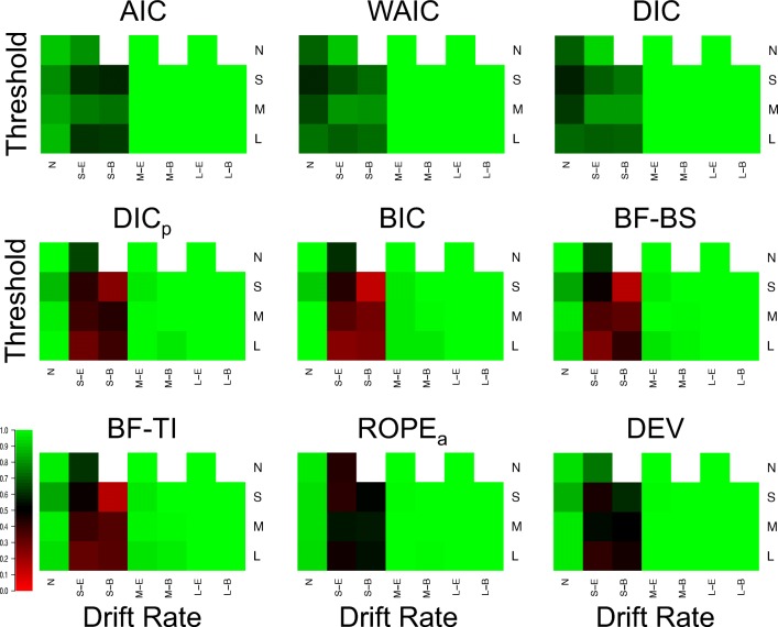
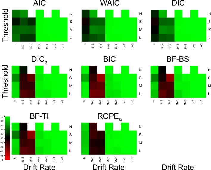
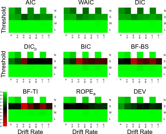
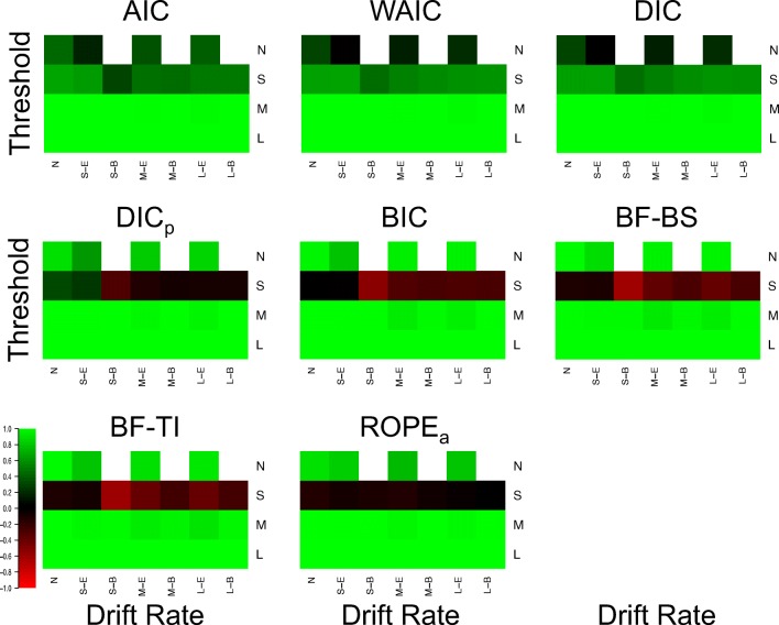
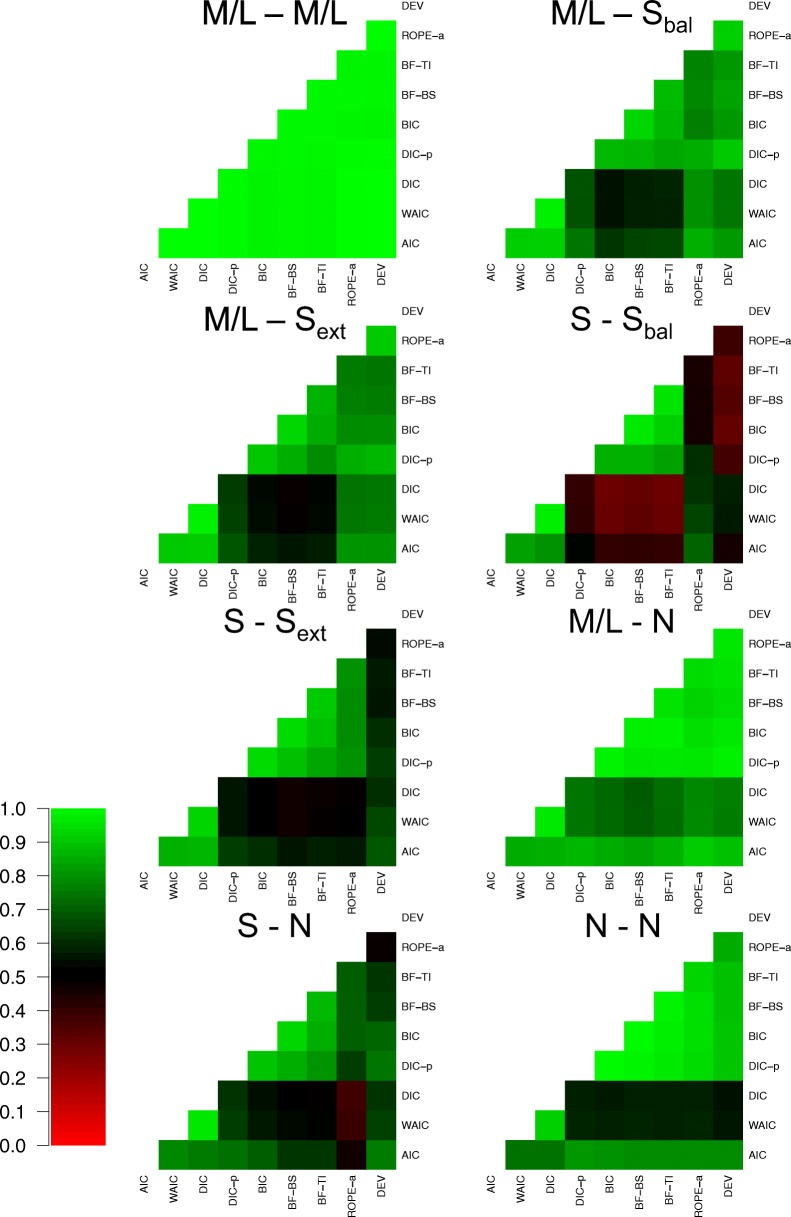
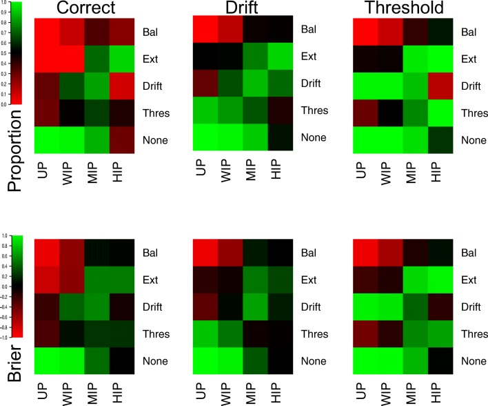
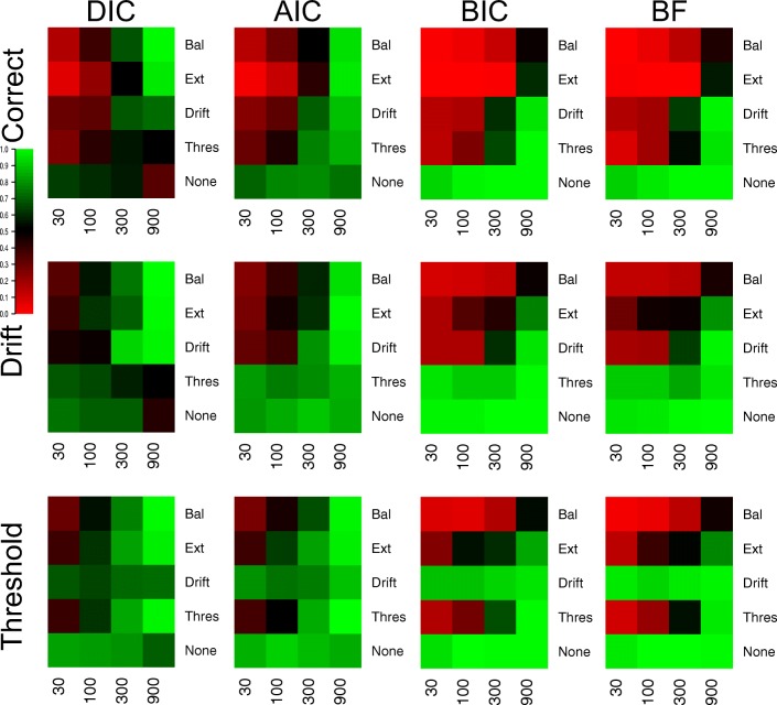
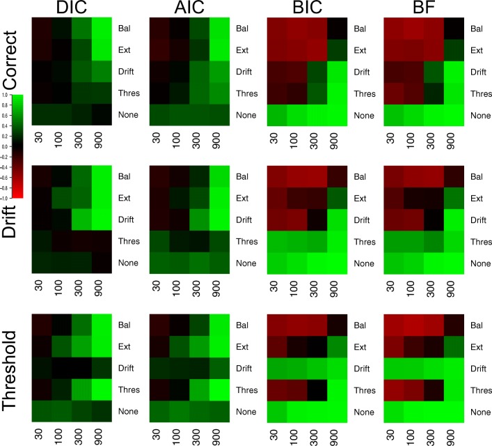
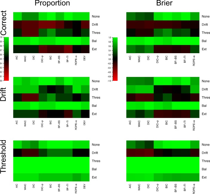
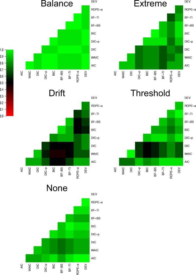
Evidence accumulations models (EAMs) have become the dominant modeling framework within rapid decision-making, using choice response time distributions to make inferences about the underlying decision process. These models are often applied to empirical data as "measurement tools", with different theoretical accounts being contrasted within the framework of the model. Some method is then needed to decide between these competing theoretical accounts, as only assessing the models on their ability to fit trends in the empirical data ignores model flexibility, and therefore, creates a bias towards more flexible models. However, there is no objectively optimal method to select between models, with methods varying in both their computational tractability and theoretical basis. I provide a systematic comparison between nine different model selection methods using a popular EAM-the linear ballistic accumulator (LBA; Brown & Heathcote, Cognitive Psychology 57(3), 153-178 2008)-in a large-scale simulation study and the empirical data of Dutilh et al. (Psychonomic Bulletin and Review, 1-19 2018). I find that the "predictive accuracy" class of methods (i.e., the Akaike Information Criterion [AIC], the Deviance Information Criterion [DIC], and the Widely Applicable Information Criterion [WAIC]) make different inferences to the "Bayes factor" class of methods (i.e., the Bayesian Information Criterion [BIC], and Bayes factors) in many, but not all, instances, and that the simpler methods (i.e., AIC and BIC) make inferences that are highly consistent with their more complex counterparts. These findings suggest that researchers should be able to use simpler "parameter counting" methods when applying the LBA and be confident in their inferences, but that researchers need to carefully consider and justify the general class of model selection method that they use, as different classes of methods often result in different inferences.

Keywords: Bayes factors; Decision-making; Model selection; Predictive accuracy; Response time modeling.

Fig. 1

Plots of the proportion of correct selections for each model selection method (different plots) for the 25 different cells of the design (rows and columns). Lighter shades of green indicate better performance, lighter shades of red indicate worse performance, and black indicates intermediate performance, which can be seen in the color bar to the left-hand side. White indicates cells that did not exist in the simulated design. Different cells display different data-generating models, with the different columns being different generated drift rates, and the different rows being different generated thresholds. For rows and columns, ‘N’ refers to no effect, ‘S’ refers to a small effect, ‘M’ refers to a moderate effect, and ‘L’ refers to a large effect. When both effects are present (i.e., not ‘N’), ‘E’ refers to an extreme difference between conditions, whereas ‘B’ refers to a balanced difference between conditions

Fig. 2

Plots of the Brier scores of correct selections for each model selection method (different plots) for the 25 different cells of the design (rows and columns). Lighter shades of green indicate better performance, lighter shades of red indicate worse performance, and black indicates intermediate performance, which can be seen in the color bar to the left-hand side. White indicates cells that did not exist in the simulated design. Different cells display different data-generating models, with the different columns being different generated drift rates, and the different rows being different generated thresholds. For rows and columns, ‘N’ refers to no effect, ‘S’ refers to a small effect, ‘M’ refers to a moderate effect, and ‘L’ refers to a large effect. When both effects are present (i.e., not ‘N’), ‘E’ refers to an extreme difference between conditions, whereas ‘B’ refers to a balanced difference between conditions

Fig. 3

Plots of the proportion of correct selections for the drift rate effect for each model selection method (different plots) for the 25 different cells of the design (rows and columns). Lighter shades of green indicate better performance, lighter shades of red indicate worse performance, and black indicates intermediate performance, which can be seen in the color bar to the left-hand side. White indicates cells that did not exist in the simulated design. Different cells display different data-generating models, with the different columns being different generated drift rates, and the different rows being different generated thresholds. For rows and columns, ‘N’ refers to no effect, ‘S’ refers to a small effect, ‘M’ refers to a moderate effect, and ‘L’ refers to a large effect. When both effects are present (i.e., not ‘N’), ‘E’ refers to an extreme difference between conditions, whereas ‘B’ refers to a balanced difference between conditions

Fig. 4

Plots of the Brier score of correct selections for the drift rate effect for each model selection method (different plots) for the 25 different cells of the design (rows and columns). Lighter shades of green indicate better performance, lighter shades of red indicate worse performance, and black indicates intermediate performance, which can be seen in the color bar to the left-hand side. White indicates cells that did not exist in the simulated design. Different cells display different data-generating models, with the different columns being different generated drift rates, and the different rows being different generated thresholds. For rows and columns, ‘n refers to no effect, ‘S’ refers to a small effect, ‘M’ refers to a moderate effect, and ‘L’ refers to a large effect. When both effects are present (i.e., not ‘N’), ‘E’ refers to an extreme difference between conditions, whereas ‘n refers to a balanced difference between conditions

Fig. 5

Plots of the proportion of correct selections for the threshold effect for each model selection method (different plots) for the 25 different cells of the design (rows and columns). Lighter shades of green indicate better performance, lighter shades of red indicate worse performance, and black indicates intermediate performance, which can be seen in the color bar to the left-hand side. White indicates cells that did not exist in the simulated design. Different cells display different data-generating models, with the different columns being different generated drift rates, and the different rows being different generated thresholds. For rows and columns, ‘N’ refers to no effect, ‘S’ refers to a small effect, ‘M’ refers to a moderate effect, and ‘L’ refers to a large effect. When both effects are present (i.e., not ‘N’), ‘E’ refers to an extreme difference between conditions, whereas ‘B’ refers to a balanced difference between conditions

Fig. 6

Plots of the proportion of correct selections for the threshold effect for each model selection method (different plots) for the 25 different cells of the design (rows and columns). Lighter shades of green indicate better performance, lighter shades of red indicate worse performance, and black indicates intermediate performance, which can be seen in the color bar to the left-hand side. White indicates cells that did not exist in the simulated design. Different cells display different data-generating models, with the different columns being different generated drift rates, and the different rows being different generated thresholds. For rows and columns, ‘N’ refers to no effect, ‘S’ refers to a small effect, ‘M’ refers to a moderate effect, and ‘L’ refers to a large effect. When both effects are present (i.e., not ‘N’), ‘E’ refers to an extreme difference between conditions, whereas ‘B’ refers to a balanced difference between conditions

Fig. 7

Plots the agreement in selected model between each of the eight model selection methods (rows and columns of each plot) for eight different groupings of the data (different plots). Lighter shades of green indicate greater agreement, lighter shades of red indicate greater disagreement, and black indicates intermediate agreement, which can be seen in the color bar to the left-hand side. For the groupings of the data, ‘n refers to no effect, ‘S’ refers to a small effect, and ‘M/L’ refers to a moderate or large effect. The two different letters refer to whether the data were generated with both effects, one effect, or neither effect. When the data were generated with both effects, the subscript ‘bal’ refers to a balanced difference between conditions, and the subscript ‘ext’ refers to an extreme difference between conditions

Fig. 8

Plots of the correct (left panels), drift (middle panels), and threshold (right panels) selections, as proportions (top panels) and average Brier scores (bottom panels). Lighter shades of green indicate better performance, lighter shades of red indicate worse performance, and black indicates intermediate performance, which can be seen in the color bar to the left-hand side. Different rows of cells display different data-generating models, and different columns display different priors

Fig. 9

Plots of the proportion of correct (top panels), drift (middle panels), and threshold (bottom panels) selections for each model selection method (different columns of panels) for the 20 different cells of the design (rows and columns). Lighter shades of green indicate better performance, lighter shades of red indicate worse performance, and black indicates intermediate performance, which can be seen in the color bar to the left-hand side

Fig. 10

Plots of the Brier scores for the correct (top panels), drift (middle panels), and threshold (bottom panels) selections for each model selection method (different columns of panels) for the 20 different cells of the design (rows and columns). Lighter shades of green indicate better performance, lighter shades of red indicate worse performance, and black indicates intermediate performance, which can be seen in the color bar to the left-hand side

Fig. 11

Plots of the proportion (left panels) and Brier scores (right panels) of correct selections (top panels), drift rate selections (middle panels), and threshold selections (bottom panels) for each model selection method (columns) for the five different cells of the design (rows). Lighter shades of green indicate more selections, lighter shades of red indicate less selections, and black indicates intermediate performance, which can be seen in the color bar to the left-hand side

Fig. 12

Plots the agreement in selected model between each of the eight model selection methods (rows and columns of each plot) for five cells of the design. Lighter shades of green indicate greater agreement, lighter shades of red indicate greater disagreement, and black indicating intermediate agreement, which can be seen in the color bar to the left-hand side

References

1. Akaike H. A new look at the statistical model identification. IEEE Transactions on Automatic Control. 1974;19(6):716–723.
1. Annis, J., Evans, N.J., Miller, B.J., & Palmeri, T.J. (2018). Thermodynamic integration and steppingstone sampling methods for estimating Bayes factors: A tutorial. Retrieved from https://psyarxiv.com/r8sgn - PMC - PubMed
1. Boehm, U., Marsman, M., Matzke, D., & Wagenmakers, E.-J. (2018). On the importance of avoiding shortcuts in applying cognitive models to hierarchical data. Behavior Research Methods, 1–18. - PMC - PubMed
1. Box GE, Draper NR. Empirical model-building and response surfaces. New York: Wiley; 1987.
1. Brier GW. Verification of forecasts expressed in terms of probability. Monthey Weather Review. 1950;78(1):1–3.
LinkOut - more resources