The single-cell transcriptional landscape of mammalian organogenesis

Abstract

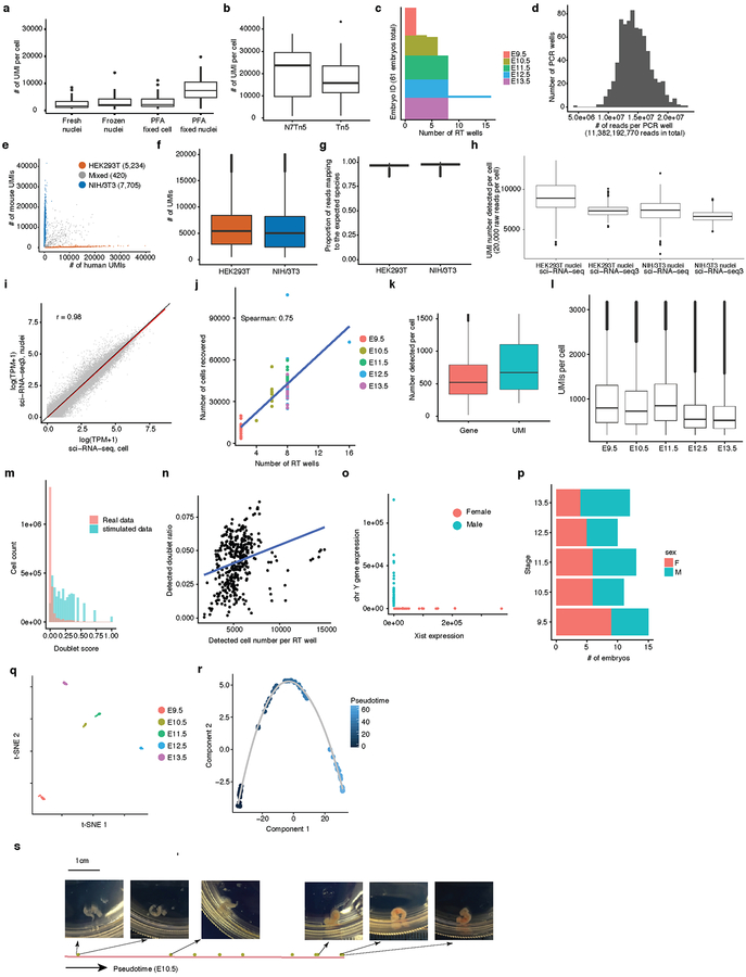
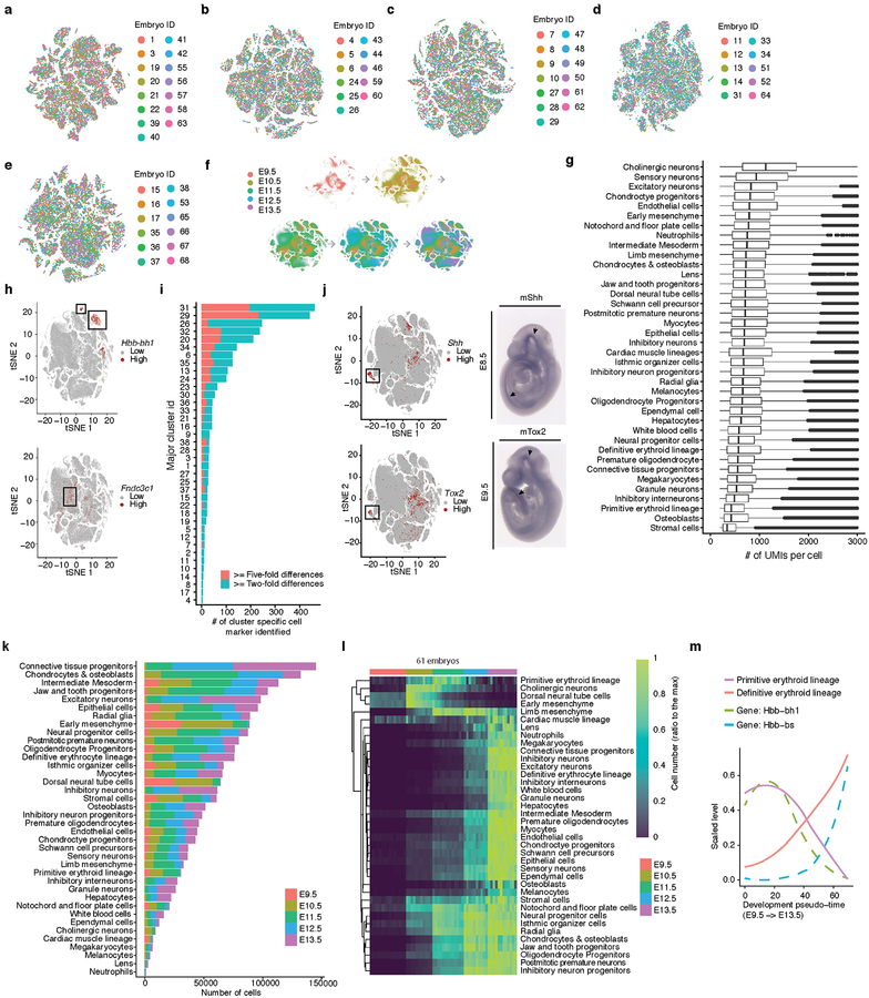
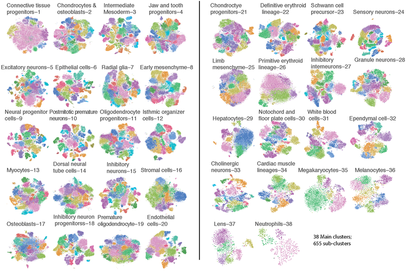
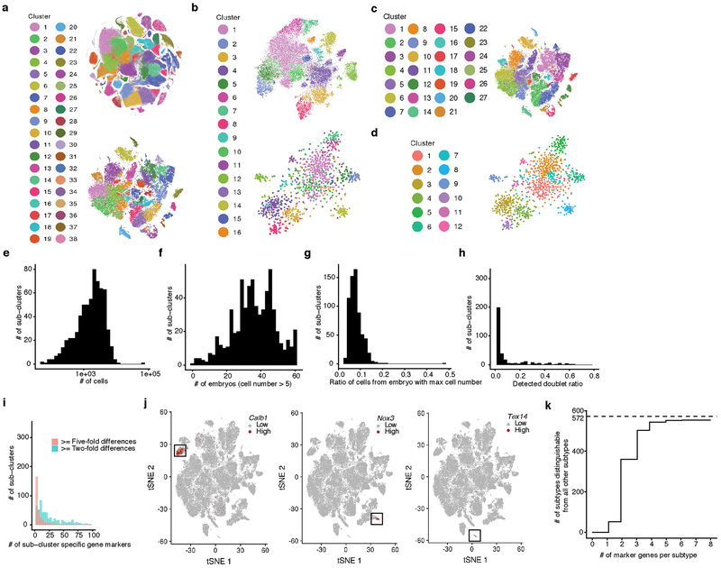
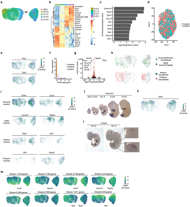
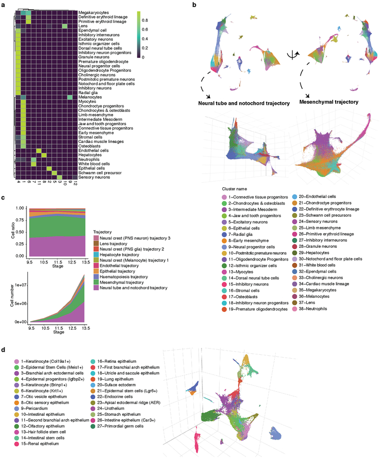
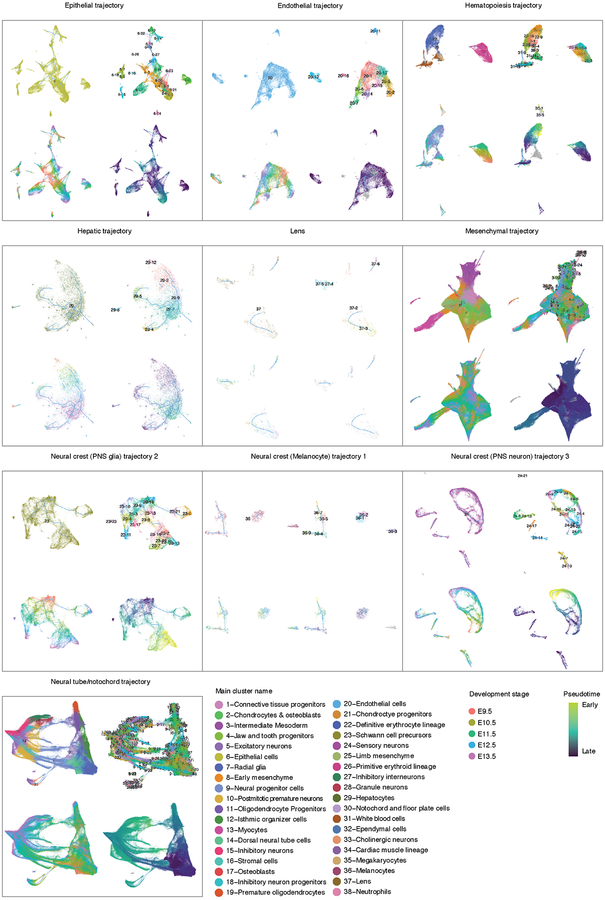
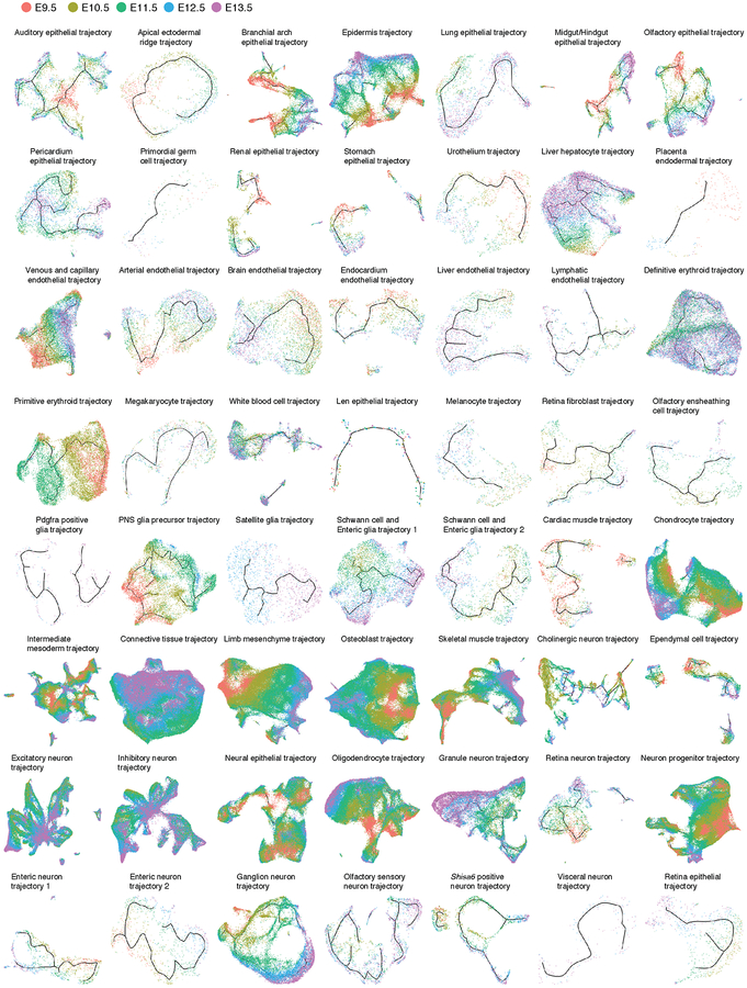
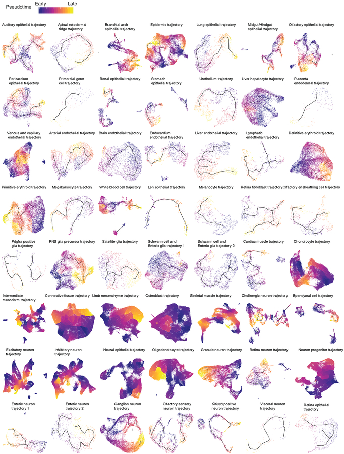
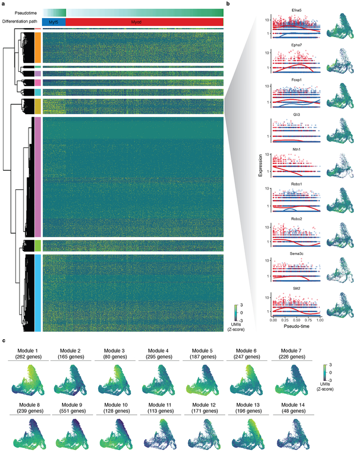
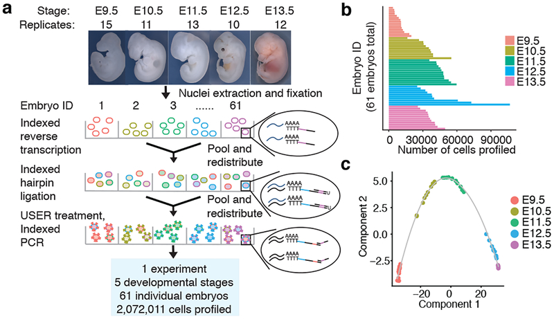
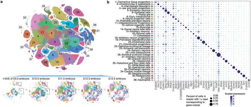
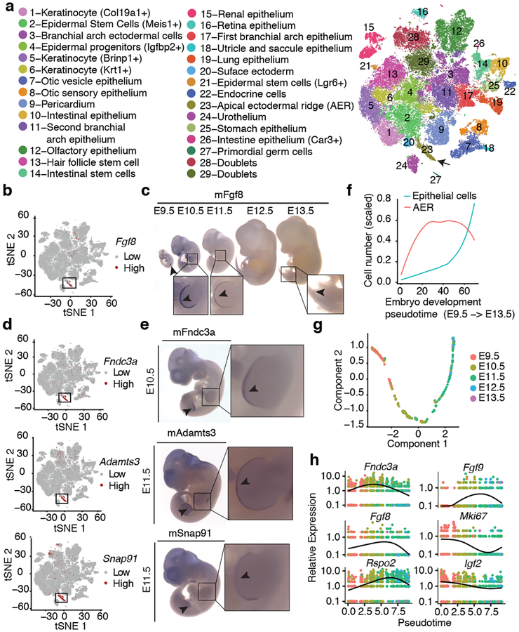
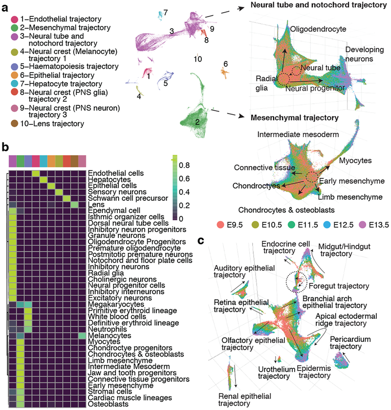
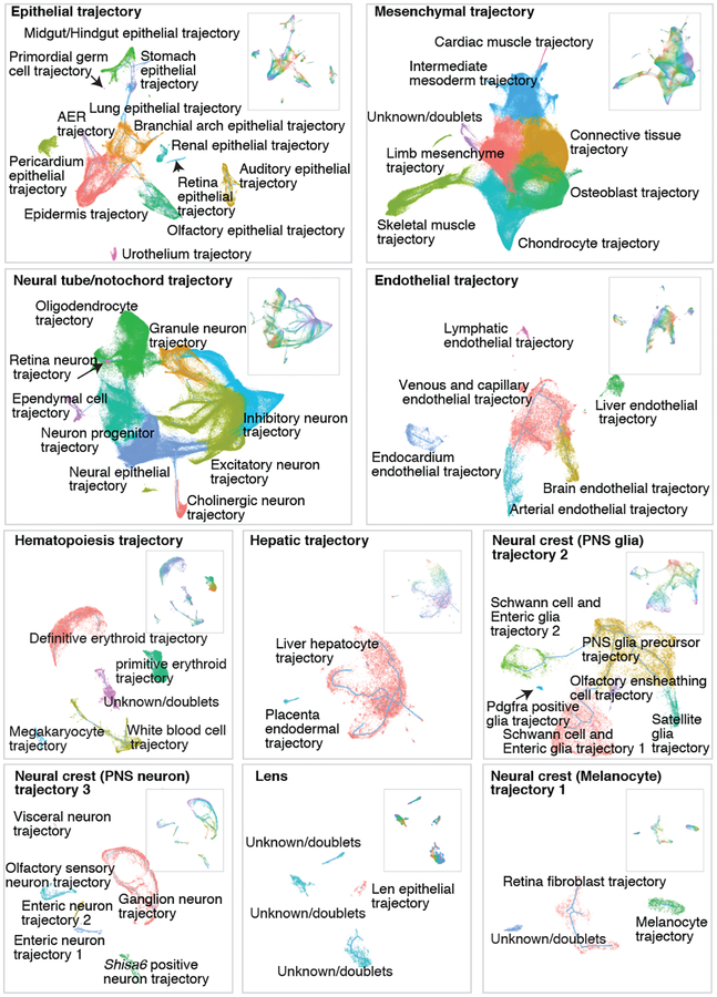
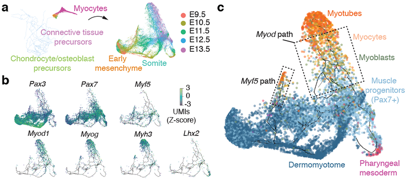
Mammalian organogenesis is a remarkable process. Within a short timeframe, the cells of the three germ layers transform into an embryo that includes most of the major internal and external organs. Here we investigate the transcriptional dynamics of mouse organogenesis at single-cell resolution. Using single-cell combinatorial indexing, we profiled the transcriptomes of around 2 million cells derived from 61 embryos staged between 9.5 and 13.5 days of gestation, in a single experiment. The resulting 'mouse organogenesis cell atlas' (MOCA) provides a global view of developmental processes during this critical window. We use Monocle 3 to identify hundreds of cell types and 56 trajectories, many of which are detected only because of the depth of cellular coverage, and collectively define thousands of corresponding marker genes. We explore the dynamics of gene expression within cell types and trajectories over time, including focused analyses of the apical ectodermal ridge, limb mesenchyme and skeletal muscle.

Extended Data Fig. 1.. Performance and QC-related analyses for sci-RNA-seq3.

(a) Comparison of fixation conditions in human HEK293T cells. Paraformaldehyde (PFA) fixed nuclei yielded the highest numbers of UMIs. Cell number n = 21 for fresh nuclei, 17 for frozen nuclei, 32 for PFA fixed cell, 31 for PFA fixed nuclei. (b) Tn5 transposomes loaded only with N7 adaptor (cell number n = 13) increased UMI counts by over 50%, relative to the standard Nextera Tn5 (cell number n = 11), in human HEK293T cells. (c) Bar plot showing the number of RT wells used for each of 61 mouse embryos. (d) Histogram showing the distribution of raw sequencing reads from each PCR well in sci-RNA-seq3. (e) Scatter plot of mouse (NIH/3T3) vs. human (HEK293T) UMI counts per cell. (f-g) Box plot showing the number of UMIs and purity (proportion of reads mapping to the expected species) per cell from HEK293T (cell number n = 7,943) and NIH/3T3 cells (cell number n = 10,914). At a sequencing depth of 23,207 reads per cell, we observed a median of 5,461 UMIs per HEK293T cell and 5,087 UMIs per NIH/3T3 cell, with 3.9% and 2.9% of reads per cell mapping to incorrect species, respectively. (h) Box plot comparing the number of UMIs per cell (downsampled to 20,000 raw reads per cell) for sci-RNA-seq3 (cell number n = 689 for HEK293T and 997 for NIH/3T3) vs. sci-RNA-seq (cell number n = 47 for HEK293T and 120 for NIH/3T3). (i) Correlation (Spearman’s correlation) between gene expression measurements in aggregated profiles of HEK293T from sci-RNA-seq3 nuclei vs. sci-RNA-seq cells. (j) Scatter plot showing correlation between number of RT wells used and number of cells recovered per embryo. (k) Box plot showing the number of genes and UMIs detected per cell. (l) Box plot showing the number of UMIs detected per cell from embryos across five developmental stages. Cell number n = 152,120 for E9.5; 378,427 for E10.5; 615,908 for E11.5; 475,047 for E12.5; 437,150 for E13.5. (m) Histogram showing the distribution of the cell doublet score for the actual mouse embryo data vs. doublets stimulated by Scrublet. (n) Scatter plot of the number of cells profiled per RT well and the detected doublet cell ratio. Blue line showing the linear regression line. The detected doublet cell rate was modestly correlated with number of cells profiled per well during reverse transcription (Spearman’s rho: 0.35). (o) Scatter plot of unique reads aligning to Xist (female-specific) vs. chrY transcripts (male-specific) per mouse embryo. Sex assignments of individual embryos inferred from these data. (p) Bar plot showing the number of male and female embryos profiled at each developmental stage. (q) t-SNE of the aggregated transcriptomes of single cells derived from each of 61 mouse embryos results in five tightly clustered groups perfectly matching their developmental stages (embryo number n = 61). (r) Pseudotime trajectory of pseudobulk RNA-seq profiles of mouse embryos (embryo number n = 61); identical to Fig. 1f, but colored by pseudotime. (s) The 61 profiled embryos were ordered by pseudotime. The three earliest vs. three latest (in pseudotime) E10.5 embryos are shown in photos, and appear to potentially be morphologically distinct. Notably, the distinct coloring of E10.5 embryos positioned earlier vs. later in developmental pseudotime is potentially due to different levels of hemoglobin. For all box plots: thick horizontal lines, medians; upper and lower box edges, first and third quartiles, respectively; whiskers, 1.5 times the interquartile range; circles, outliers.

Extended Data Fig. 2.. Identifying the major cell types and cell composition dynamics during mouse organogenesis.

(a-e) t-SNE visualization of mouse embryo cells from different developmental stages, as shown in lower portion of Fig. 2a, but sampling 10,000 cells per stage and coloring by embryo ID: E9.5 (a), E10.5 (b), E11.5 (c), E12.5 (d), E13.5 (e). We consistently observe that cells derived from independent embryos at the same timepoint are similarly distributed. (f) The same t-SNE as Fig. 2a is shown, with subsets of cells highlighted. The first panel only shows cells from E9.5 embryos, and cells from subsequent developmental stages are progressively added. (g) Box plot showing the number of UMIs detected per cell for major cell types (cell number n for each cell type is listed in Supplementary Table 3). Thick horizontal lines, medians; upper and lower box edges, first and third quartiles, respectively; whiskers, 1.5 times the interquartile range; circles, outliers. (h) t-SNE visualization of a randomly sampled 100,000 cells colored by expression level of Hbb-bh1 (top) or Fndc3c1 (bottom). “High” indicates cells with UMI count for Hbb-bh1 > 3, Fndc3c1 > 1. (i) Bar plot showing the number of marker genes in each major cell type, defined as differentially expressed genes (5% FDR) with a >2-fold (green) or >5-fold (red) expression difference between first and second ranked cell types. (j) Left: t-SNE visualization of a randomly sampled 100,000 cells colored by expression level of Shh (top) or Tox2 (bottom). Right: whole mount in situ hybridization images of Shh (top) or Tox2 (bottom) in embryos. n = 5 “High” indicates cells with UMI count for Shh > 0, Tox2 > 1. Arrow: site of gene expression. (k) Bar plot showing the number of cells profiled for each cell type, split out by development stage. (l) Heatmap showing the estimated relative number of each cell type (rows) in 61 mouse embryos (columns). An estimate of the absolute cell number per cell type per embryo was calculated by multiplying the proportion that cell type contributed to a given embryo by the estimated total number of cells at that development stage. For presentation, these estimates are normalized in each row by the maximum estimated cell count for that cell type across all 61 embryos. Embryos are sorted left-to-right by developmental pseudotime. (m) Line plot showing the estimated relative cell numbers for primitive erythroid and definitive erythroid lineages, calculated as in panel b. Dashed lines show relative expression of marker genes for primitive erythroid (Hbb-bh1) and definitive erythroid (Hbb-bs) major cell types. Data points for individual embryos were ordered by development pseudotime and smoothed by the loess method.

Extended Data Fig. 3.. Louvain clustering and t-SNE visualization of subclusters of the each of 38 major cell types.

As cell type heterogeneity was readily apparent within many of the 38 clusters shown in Fig. 2a, we adopted an iterative strategy, repeating Louvain clustering on each main cell type to identify subclusters. After subclusters dominated by one or two embryos were removed and highly similar subclusters merged, a total of 655 subclusters (also termed ‘subtypes’ to distinguish them from the 38 major cell types identified by the initial clustering). Cell number n for each cell type is listed in Supplementary Table 3.

Extended Data Fig. 4.. Analysis of cell subtypes during mouse organogenesis.

(a) t-SNE visualization of all cells (top plot, n = 2,026,641) and downsampled subset of high-quality cells (bottom plot, n = 50,000, UMI > 400), colored by Louvain cluster IDs from Fig. 2a. (b) t-SNE visualization of all endothelial cells (top plot, n = 35,878) and those from the downsampled subset (bottom plot, n = 1,173), colored by Louvain cluster ID computed based on the 35,878 endothelial cells. (c-d) t-SNE visualization of the downsampled subset of 50,000 cells (c), and 1,173 endothelial cells (d), colored by Louvain cluster ID computed based on sampled cells only. The number of clusters and subclusters identified with the same parameters drops from 38 (a, bottom plot) to 27 (c) and 16 (b, bottom plot) to 12 (c), respectively. (e) Histogram showing the distribution of subclusters with respect to cell number (median 1,869; range 51–65,894). (f) Histogram showing the distribution of subclusters with respect to the number of contributing embryos (>5 cells to qualify as a contributor). (g) Histogram showing the distribution of subclusters with respect to the ratio of cells derived from the most highly contributing embryo. (h) Histogram showing the distribution of subclusters with respect to the ratio of doublet cells detected by Scrublet. (i) Histogram showing the distribution of subclusters with respect to the number of marker genes (at least 2-fold (blue) or 5-fold (red) higher expression when compared with the second highest expressing cell subtype within the same main cluster; 5% FDR). 644 of 655 sub-clusters (98%) have at least one such gene marker with a 2-fold difference, and 441 of 655 (67%) have at least one such marker with a 5-fold difference. (j) t-SNE visualization of subcluster specific marker expression (as example, cell number n = 74,651): Calb1 (left), Nox3 (middle) and Tex14 (right) are gene markers for three endothelial subclusters. “High” indicates cells with UMI count for Calb1 > 0, Nox3 > 0, Tex14 >1. (k) Cumulative histogram showing how many subtypes (out of a total of 572 non-doublet-artifact subtypes) can be distinguished from all other subtypes on the basis of one or several markers and >4-fold expression differences (see also Methods, Supplementary Table 5).

Extended Data Fig. 5.. Cell type correlation analysis between single cell mouse atlases.

(a) Cell type correlation analysis (Methods) matched cell types between independently generated and annotated analyses of the adult mouse kidney (sci-RNA-seq component of sci-CAR (rows) vs. Microwell-seq (columns)). All cell types identified by sci-RNA-seq are shown, but we only show Microwell-seq cell types that are top matches for 1+ sci-RNA-seq cell types. Colors correspond to beta values, normalized by the maximum beta value per row. (b) Left: We compared our subtypes against 130 fetal cell types annotated in the MCA with cell type correlation analysis, matching 96 MCA-defined cell types (rows) to 58 subtypes in our mouse embryo atlas (columns). Colors correspond to beta values, normalized by the maximum beta value per row. All MCA cell types with maximum beta of matched cell type > 0.01 are shown (rows; n = 96), as are mouse embryo atlas cell types that are top matches for 1+ displayed MCA cell types (columns; n = 58). Right: zoom-in to a subset of matches shown on the left. Cell types annotations are from MCA (rows) or our study (columns; major cell type annotation and sub-cluster id). (c) Box plot showing the ratio of cells from E13.5 for subclusters with (sub-cluster number n = 58) vs. without (sub-cluster number n = 514) a matched cell type in the MCA. Thick horizontal lines, medians; upper and lower box edges, first and third quartiles, respectively; whiskers, 1.5 times the interquartile range; circles, outliers. (d) Left: We compared our subtypes against 265 cell types annotated by a recent mouse brain cell atlas (BCA) with cell type correlation analysis, matching 48 BCA-defined cell types (rows) to 68 subtypes in our data (columns). Colors correspond to beta values, normalized by the maximum beta value per row. All mouse embryo cell types with maximum beta of matched cell type > 0.01 are shown (column; n = 68), as are BCA cell types that are top matches for 1+ displayed mouse embryo cell types (rows; n = 48). Right: zoom-in to a subset of matches shown on the left. Cell types annotations are from BCA (rows) or our study (columns; major cell cluster and sub-cluster id).

Extended Data Fig. 6.. Analysis of mouse epithelium, endothelium and limb apical ectodermal ridge cells.

(a-b) Dot plot showing expression of one selected marker gene per epithelial (a) or endothelial (b) subtype. Doublet-derived subclusters (2/29 epithelial subtypes and 5/16 endothelial subtypes) are excluded from these plots, but are still shown in Fig. 3a and panel c, respectively. The size of the dot encodes the percentage of cells within a cell type, and its color encodes the average expression level. (c) t-SNE visualization and marker-based annotation of endothelial cell subtypes (n = 35,878). (d) Heatmap showing smoothed pseudotime-dependent differential gene expression (169 genes at FDR of 1%) in AER cells, generated by a spline fitting with generalized linear model (assuming gene expression following the negative binomial distribution) and scaled as a percent of maximum gene expression. Each row indicates a different gene, and these are split into subsets that are activated (top), repressed (middle) or exhibit transient dynamics (bottom) between E9.5 and E13.5. (e-f) Plots showing the −log10 transformed q value and Enrichr based combined score of enriched Reactome terms (e) and transcription factors (f) for genes whose expression significantly decreases in AER development. The top enriched pathway terms (Reactome2016) for significantly decreasing genes include cell cycle progression (Mitotic Cell Cycle, qval = 0.0002, one-sided Fisher exact test with multiple comparisons adjusted) and glucose metabolism (Metabolism of carbohydrates, qval = 0.0002, one-sided Fisher exact test with multiple comparisons adjusted). The top enriched TFs with targets from decreasing genes include pluripotent factors such as Isl1 (qval < 1e-5), Pou5f1 (qval = 0.002, one-sided Fisher exact test with multiple comparisons adjusted) and Nanog (qval = 0.003, one-sided Fisher exact test with multiple comparisons adjusted).

Extended Data Fig. 7.. Characterizing cellular trajectories during limb mesenchyme differentiation.

(a) UMAP 3D visualization of limb mesenchymal cells colored by development stage (cell number n = 26,559, left and right represent views from two directions). (b) Heatmap showing top differentially expressed genes between different developmental stages for limb mesenchyme cells. (c) Bar plot showing the −log10 transformed adjusted p value (one-sided Fisher exact test with multiple comparisons adjusted) of enriched transcription factors for significantly up-regulated genes during limb mesenchyme development. (d) t-SNE visualization of limb mesenchyme cells colored by forelimb (Tbx5 +, cell number n = 2,085) and hindlimb (Pitx1+, cell number n = 1,885). Cells with no expression or both expression in Tbx5 and Pitx1 are not shown. (e, h, i, k) Each panel illustrates a different marker gene. Colors indicate UMI counts that have been scaled for library size, log-transformed, and then mapped to Z-scores to enable comparison between genes. Cells with no expression of a given marker are excluded to prevent overplotting. (e) Hindlimb marker Pitx1 and forelimb marker Tbx5. (f) Scatter plot showing the normalized expression of Pitx1 and Tbx5 in limb mesenchyme cells. Only cells in which Pitx1 and/or Tbx5 detected were shown. (g) Volcano plot showing the differentially expressed genes (FDR of 5%, one-sided likelihood ratio test with multiple comparisons adjusted, colored by red) between forelimb (cell number n = 2,085) and hindlimb (cell number n = 1,885). Top differentially expressed genes are labeled. X axis: log2 transformed fold change between forelimb and hindlimb for each gene. Y axis: −log10 transformed qval from differential gene expression test. (h) Same visualization as panel e, colored by normalized gene expression of proximal/chondrocyte (Sox6, Sox9), distal (Hoxd13, Tfap2b), anterior (Pax9, Alx4), or posterior (Hand2, Shh) markers. Only cells with the gene marker expressed are plotted. (i) Same visualization as panel e. First row: proximal limb markers Sox6 (which also marks chondrocytes) and Sox9. Second row: distal limb markers Hoxd13 and Tfap2b. Third row: Anterior limb markers Pax9 and Alx4. Fourth row: posterior limb markers Shh and Hand2. (j) In situ hybridization images of Hoxd13 in E9.5 to E13.5 embryos, n = 5. (k) Same visualization as panels e, colored by normalized gene expression of Cpa2. Only cells with positive UMI counts are shown. Values are log10-transformed, standardized UMI counts. Its expression pattern within this trajectory led us to predict that Cpa2 is a distal marker of the developing limb mesenchyme, like Hoxd13. (l) In situ hybridization images of Cpa2 in E10.5 and E11.5 embryos, n = 5. Arrow: site of gene expression. (m) Modules of spatially restricted genes in the limbs. A total of 1,783 genes were clustered via hierarchical clustering. The dendrogram was cut into 8 modules using the cutree function in R, and the aggregate expression of genes in each module was computed. Colors indicate aggregate UMI counts for each module that have been scaled for library size, log-transformed, and then mapped to Z-scores to enable comparison between modules. Cells with no expression of a given module are excluded to prevent overplotting.

Extended Data Fig. 8.. Characterization of ten major developmental trajectories present during mouse organogenesis.

(a) Heatmap showing the proportion of cells from each of the 38 major cell types assigned to each of the twelve PAGA algorithm-identified groups. We merged two groups corresponding to sensory neurons (12 & 3), and another two groups corresponding to blood cells (6 & 7), as each pair was closely located in UMAP space upon visual inspection, yielding the ten supergroups shown in a similar heatmap in Fig. 4b. (b) Same as Fig. 4a, but with colors corresponding to the 38 major cell clusters. (c) Area plot showing the estimated proportion (top) and estimated absolute number (bottom) of cells per embryo derived from each of the ten major cell trajectories from E9.5 to E13.5. Although the estimated number of cells per embryo in each of these supergroups increases exponentially, their proportions remain relatively stable, with the exception of hepatocytes which expand their contribution by nearly ten-fold during this developmental window (from 0.3% at E9.5 to 2.8% at E13.5). (d) UMAP 3D visualization of epithelial subtrajectories (as in Fig. 4c), colored as per the epithelial subtypes shown in Fig. 3a.

Extended Data Fig. 9.. UMAP visualization of the ten major cell trajectories.

We iteratively reanalyzed each of the ten major trajectories, nearly all of which further resolved into multiple subtrajectories. The ten major cell trajectories are visualized with UMAP (as in Fig. 5) but colored: as per the 38 major cell clusters (top left), sub-cluster id (top right), developmental stage (bottom left) and pseudotime (bottom right). The lines correspond to the principal graph learned by Monocle 3. These images are also available at http://atlas.gs.washington.edu/mouse-rna/3dplot/ as manipulatable 3D renderings.

Extended Data Fig. 10.. UMAP visualization of the 56 subtrajectories, colored by development stage.

We further iteratively reanalyzed and visualized with UMAP each of the 56 subtrajectories. Although Monocle 3 did not have access to these labels, the subtrajectories are highly consistent with developmental time (i.e. cells ordered from E9.5 to E13.5). The lines correspond to the principal graph learned by Monocle 3.

Extended Data Fig. 11.. UMAP visualization of the 56 subtrajectories, colored by inferred pseudotime.

To orient each subtrajectory (same projections as Extended Data Fig. 10), we identified one or several starting points as focal concentrations of E9.5 cells, and then computed developmental pseudotime for cells present along various paths. The lines correspond to the principal graph learned by Monocle 3.

Extended Data Fig. 12.. Gene dynamics in the myogenic trajectory.

(a) Genes that are differentially expressed between the Myf5 path and the Myod path highlighted in Fig. 6. Cells along each path were compared via Monocle’s differentialGeneTest function. Pseudotimes along each path were scaled from 0 to 100 independently. The “full model” formula was “~path * sm.ns(Pseudotime, df=3)”, while the “reduced model” was “~sm.ns(Pseudotime, df=3)”. Differentially expressed genes (FDR < 1%, one-sided likelihood ratio test with multiple comparisons adjusted) were clustered via Ward’s method and visualized as a heatmap via the pheatmap package. (b) Pseudotemporal kinetics for selected genes involved in Robo/Slit signaling. Red indicates cells on the Myod path, while blue corresponds to the Myf5 path. Next to the expression curves for each are shown the standardized expression scores for each gene on the original myogenic trajectory. Only cells with detectable expression are rendered to prevent overplotting. (c) Modules of genes differentially expressed over the myogenic trajectory. A total of 2,908 genes were clustered via hierarchical clustering. The dendrogram was cut into 14 modules using the cutree function in R, and the aggregate expression of genes in each module was computed. Colors indicate aggregate UMI counts for each module that have been scaled for library size, log-transformed, and then mapped to Z-scores to enable comparison between modules. Cells with no expression of a given module are excluded to prevent overplotting.

Fig. 1.. sci-RNA-seq3 enables profiling of 2,072,011 cells from 61 mouse embryos across 5 developmental stages in a single experiment.

(a) sci-RNA-seq3 workflow and experimental scheme. (b) Bar plot showing number of cells profiled from each of 61 mouse embryos. (c) Pseudotime trajectory of pseudobulk RNA-seq profiles of mouse embryos.

Fig. 2.. Identifying the major cell types of mouse organogenesis.

(a) t-SNE visualization of 2,026,641 mouse embryo cells, colored by cluster id from Louvain clustering (in Fig. 2b), and annotated based on marker genes. The same t-SNE is plotted below, showing only cells from each stage (cell numbers from left to right: n = 151,000 for E9.5; 370,279 for E10.5; 602,784 for E11.5; 468,088 for E12.5; 434,490 for E13.5). Primitive erythroid (transient) and definitive erythroid (expanding) clusters are boxed. (b) Dot plot showing expression of one selected marker gene per cell type. The size of the dot encodes the % of cells within a cell type in which that marker was detected, and its color encodes the average expression level.

Fig. 3.. Identification and characterization of epithelial cell subtypes and the limb apical ectodermal ridge (AER).

(a) t-SNE visualization and marker-based annotation of epithelial cell subtypes (74,651 cells). (b) t-SNE visualization of all epithelial cells colored by expression level of Fgf8. “High” indicates cells with UMI count for Fgf8 > 1. (c) In situ hybridization images of Fgf8 in embryos from E9.5 to E13.5. Arrow: site of gene expression. n = 5 (d, e) t-SNE visualization of all epithelial cells colored by expression level (d) and whole in situ hybridization images (e) of Fndc3a (top), Adamts3 (middle) and Snap91 (bottom). n = 5 “High” indicates cells with UMI count for Fndc3a > 3, Adamts3 > 1, Snap91 > 1. Arrow: site of gene expression. (f) Line plot showing the estimated relative cell numbers for epithelial cells and AER cells, calculated as in Extended Data Fig. 2m. Data points for individual embryos were ordered by development pseudotime and smoothed by loess method. (g) Pseudotime trajectory of AER single cell transcriptomes (cell number n = 1,237), colored by development stage. (h) Kinetics plot showing relative expression of AER marker genes across developmental pseudotime.

Fig. 4.. Characterization of ten major developmental trajectories present during mouse organogenesis.

(a) UMAP 3D visualization of our overall dataset; left: views from one direction; bottom: zoomed view of neural tube/notochord (top) and mesenchymal (bottom) trajectories, colored by development stage. PNS: peripheral nervous system. (b) Heatmap showing the proportion of cells from each of the 38 major cell types (rows) assigned to each of the 10 major trajectories (columns; color key in left panel of a). (c) UMAP 3D visualization of epithelial subtrajectories colored by development stage (color key in right panel of a).

Fig. 5.. UMAP visualization of individual major trajectories.

After removing doublet-annotated cells and subclusters, we iteratively reanalyzed each of the ten major trajectories. Colored by subtrajectory name (main plots) or developmental stage (insets; colors as in Fig. 4c). Edges in the principal graphs that define trajectories reported by Monocle 3 are shown as light blue line segments.

Fig. 6.. Resolving cellular trajectories in myogenesis.

Edges in the principal graphs that define trajectories reported by Monocle 3 are shown as light blue line segments. (a) Cells putatively involved in myogenesis were isolated from the mesenchymal cell trajectory in silico and then used to construct a myocyte subtrajectory. Principal graph nodes with more than 50% occupied by cells from cluster 13 were taken as “seed nodes” and then cells on any nodes within 20 edges of these seed nodes were selected for subtrajectory analysis. Cells in the myocyte subtrajectory (left) colored by developmental stage (right). (b) Cells in the myocyte trajectory, colored by their expression of selected transcriptional regulators of myogenesis. Cells with no detectable expression for a given gene are omitted from its plot. Values are log10-transformed, standardized UMI counts. (c) Cells classified by developmental stage according to the markers shown in panel c (Dermomyotome: Pax3+, Pax7-; Muscle progenitors: Pax7+; Myoblasts: Myf5+ or Myod+ and Myog-; Myocytes: Myog+; Myotubes: Myh3+).

References

1. Kojima Y, Tam OH & Tam PPL Timing of developmental events in the early mouse embryo. Semin. Cell Dev. Biol 34, 65–75 (2014). - PubMed
1. Tam PPL & Loebel DAF Gene function in mouse embryogenesis: get set for gastrulation. Nat. Rev. Genet 8, 368–381 (2007). - PubMed
1. Dickinson ME et al. High-throughput discovery of novel developmental phenotypes. Nature 537, 508–514 (2016). - PMC - PubMed
1. Meehan TF et al. Disease model discovery from 3,328 gene knockouts by The International Mouse Phenotyping Consortium. Nat. Genet 49, 1231–1238 (2017). - PMC - PubMed
1. Wagner DE et al. Single-cell mapping of gene expression landscapes and lineage in the zebrafish embryo. Science 360, 981–987 (2018). - PMC - PubMed
Methods References
1. Li D et al. Formation of proximal and anterior limb skeleton requires early function of Irx3 and Irx5 and is negatively regulated by Shh signaling. Dev. Cell 29, 233–240 (2014). - PubMed
1. Kraft K et al. Deletions, Inversions, Duplications: Engineering of Structural Variants using CRISPR/Cas in Mice. Cell Rep (2015). doi: 10.1016/j.celrep.2015.01.016 - DOI - PubMed
1. Buenrostro JD, Giresi PG, Zaba LC, Chang HY & Greenleaf WJ Transposition of native chromatin for fast and sensitive epigenomic profiling of open chromatin, DNA-binding proteins and nucleosome position. Nat. Methods 10, 1213–1218 (2013). - PMC - PubMed
1. Renaud G, Stenzel U, Maricic T, Wiebe V & Kelso J deML: robust demultiplexing of Illumina sequences using a likelihood-based approach. Bioinformatics 31, 770–772 (2015). - PMC - PubMed
1. Dobin A et al. STAR: ultrafast universal RNA-seq aligner. Bioinformatics 29, 15–21 (2013). - PMC - PubMed
Publication types