The evolution of phenotypic plasticity when environments fluctuate in time and space

Abstract

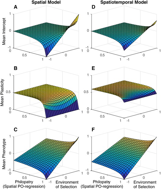
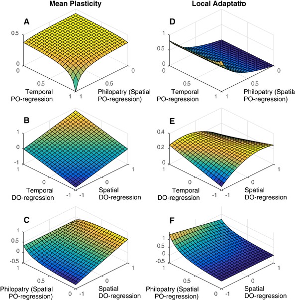
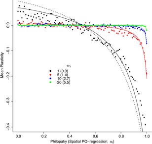
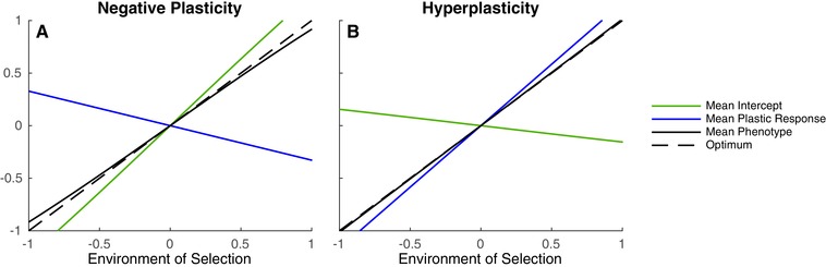
Most theoretical studies have explored the evolution of plasticity when the environment, and therefore the optimal trait value, varies in time or space. When the environment varies in time and space, we show that genetic adaptation to Markovian temporal fluctuations depends on the between-generation autocorrelation in the environment in exactly the same way that genetic adaptation to spatial fluctuations depends on the probability of philopatry. This is because both measure the correlation in parent-offspring environments and therefore the effectiveness of a genetic response to selection. If the capacity to genetically respond to selection is stronger in one dimension (e.g., space), then plasticity mainly evolves in response to fluctuations in the other dimension (e.g., time). If the relationships between the environments of development and selection are the same in time and space, the evolved plastic response to temporal fluctuations is useful in a spatial context and genetic differentiation in space is reduced. However, if the relationships between the environments of development and selection are different, the optimal level of plasticity is different in the two dimensions. In this case, the plastic response that evolves to cope with temporal fluctuations may actually be maladaptive in space, resulting in the evolution of hyperplasticity or negative plasticity. These effects can be mitigated by spatial genetic differentiation that acts in opposition to plasticity resulting in counter-gradient variation. These results highlight the difficulty of making space-for-time substitutions in empirical work but identify the key parameters that need to be measured in order to test whether space-for-time substitutions are likely to be valid.

Keywords: Counter‐gradient variation; environmental heterogeneity; hyperplasticity; local adaptation; phenotypic plasticity; space; time.

Figure 1

Island mean reaction norm components averaged over time and the environment of development, as functions of the spatial component of the environment of selection $S_i$ and the probability of philopatry ${\alpha }_I$. The intercepts are represented in the first row (a,d), the plastic slopes in the second row (b,e) and the phenotype in third row (c,f). The left column (a‐c) represents a model where only spatial variation exists, such that any environmental variation in time is absent (${\sigma }_{D_T}^2={\sigma }_{S_T}^2=0$), and the right column (d‐f) a model where spatial and temporal variation exist simultaneously (${\sigma }_{D_T}^2={\sigma }_{S_T}^2=1$). From the assumption that environmental fluctuations specific to a time and place are zero, ${\sigma }_{D_{I·T}}^2={\sigma }_{S_{I·T}}^2=0$. The remaining fixed parameters are ${\sigma }_{D_I}^2={\sigma }_{S_I}^2=1$ $A=0$, $B=1$, $G_{aa}=G_{bb}=E_{aa}=E_{bb}=1$, ${\omega }_z=1$, ${\omega }_b=3$, ${\kappa }_I={\kappa }_T=0.8$, ${\alpha }_T=0.5$.

Figure 2

Mean plasticity (left column) and local adaptation (right column) as functions of model parameters. (A) and (B) show that the spatial and temporal parameters have a symmetric effect on mean plasticity and (C) demonstrates what happens when the spatial parameters are allowed to vary but the temporal parameters are fixed (${\kappa }_T=0.5$, ${\alpha }_T=0.5$, and ${\sigma }_{D_T}^2=1$). How genetic tracking in space (the between island covariance between the intercept and the environment of selection) depends on the PO‐regressions and DO‐regressions are shown in (D) and (E), respectively. (F) shows how genetic tracking in space depends on spatial parameters when temporal parameters are fixed. The remaining fixed parameter values are $A=0$, $B=1$, $G_{aa}=E_{aa}=1$, $G_{bb}=E_{bb}=0$, ${\omega }_z=1$, ${\omega }_b=3$, ${\sigma }_{D_T}^2={\sigma }_{D_I}^2={\sigma }_{S_T}^2={\sigma }_{S_I}^2=1$, and $S_i=0$. From the assumption that environmental fluctuations specific to a time and place are zero, ${\sigma }_{D_{I·T}}^2={\sigma }_{S_{I·T}}^2=0$. Whenever constant, ${\kappa }_I=0.5$, ${\kappa }_T=0.8$, ${\alpha }_I=0.5$, and ${\alpha }_T=0.5$.

Figure 3

Mean plasticity ($\overline{b}$) in stochastic simulations with 1000 islands over 10,000 generations. A single simulation, represented by a single dot, was conducted for each of 100 migration rates $(1-{\alpha }_I)$, for four different strengths of stabilizing selection on the phenotype (${\omega }_z$; small values indicate stronger stabilizing selection), given by the different colors. The number in parentheses is the average value of ${\omega }_z$ scaled by the within‐population phenotypic variance. For comparison with the simulations, expected mean plasticities obtained using the approximation $G^{bb}\to 0$, where ${\gamma }_z$ is set to $E[{\gamma }_{z_{it}}]$, are shown for each strength of stabilizing selection. $E[{\gamma }_{z_{it}}]$ is calculated assuming no variance in slopes (dashed line) or a third‐order Taylor expansion in $D_{it}$ (solid line). Parameter values were set to ${\alpha }_T=0.5$, ${\sigma }_{D_T}^2={\sigma }_{S_T}^2={\sigma }_{D_I}^2={\sigma }_{S_I}^2=1$, $A=0$, $B=1$, $G^{aa}=E^{aa}=G^{bb}=E^{bb}=1$, ${\kappa }_T=-0.8$, ${\kappa }_I=0.8$, and ${\omega }_b=3$. From the assumption that environmental fluctuations specific to a time and place are zero, ${\sigma }_{D_{I·T}}^2={\sigma }_{S_{I·T}}^2=0$.

Figure 4

Graphical representations of negative plasticity (A) and hyperplasticity (B) across the average environment of selection of each island. Full lines correspond to island expectations of the intercept (green), effect of plasticity ($\overline{b}{D}_{it}$) (blue) and phenotype (black), averaged over time, and the dashed line corresponds to the phenotypic optimum. (A) shows that when the DO‐regression coefficient is negative in time (${\kappa }_T=-0.8$) and positive in space (${\kappa }_I=0.8$), plasticity causes a spatial change in phenotype that is opposite in sign to the change in the optimum. Environmental variances are ${\sigma }_{D_T}^2={\sigma }_{S_T}^2={\sigma }_{D_I}^2={\sigma }_{S_I}^2=1$. (B) shows that when both the DO‐regression coefficient and the environmental variances are greater in time (${\kappa }_T=2$ and ${\sigma }_{D_T}^2={\sigma }_{S_T}^2=2$) than in space (${\kappa }_I=0.8$ and ${\sigma }_{D_I}^2={\sigma }_{S_I}^2=0.05$), plasticity can evolve to values that overshoot the optimum. In both cases, if the rate of philopatry is high enough (${\alpha }_I=0.99$), subpopulations can genetically track spatial fluctuations to counteract the effects of plasticity. The remaining fixed parameter values are $A=0$, $B=1$, $G_{aa}=G_{bb}=E_{aa}=E_{bb}=1$, ${\omega }_z=1$, ${\omega }_b=3$, ${\alpha }_I=0.99$, and ${\alpha }_T=0.5$. From the assumption that environmental fluctuations specific to a time and place are zero, ${\sigma }_{D_{I·T}}^2={\sigma }_{S_{I·T}}^2=0$.

References

1. Blanquart, F. , Gandon S., and Nuismer S. L.. 2012. The effects of migration and drift on local adaptation to a heterogeneous environment. J. Evol. Biol. 25: 1351–1363. - PubMed
1. Bull, J . 1987. Evolution of phenotypic variance. Evolution 41: 303–315. - PubMed
1. van Buskirk, J . 2017. Spatially heterogeneous selection in nature favors phenotypic plasticity in anuran larvae. Evolution 71: 1670–1685. - PubMed
1. Cenzer, M. L . 2017. Maladaptive plasticity masks the effects of natural selection in the red‐shouldered soapberry bug. Am. Nat. 190: 521–533. - PubMed
1. Chevin, L.‐M. , and Lande R.. 2015. Evolution of environmental cues for phenotypic plasticity. Evolution 69: 2767–2775. - PubMed