A deep learning approach for real-time detection of sleep spindles

Abstract

Objective: Sleep spindles have been implicated in memory consolidation and synaptic plasticity during NREM sleep. Detection accuracy and latency in automatic spindle detection are critical for real-time applications.

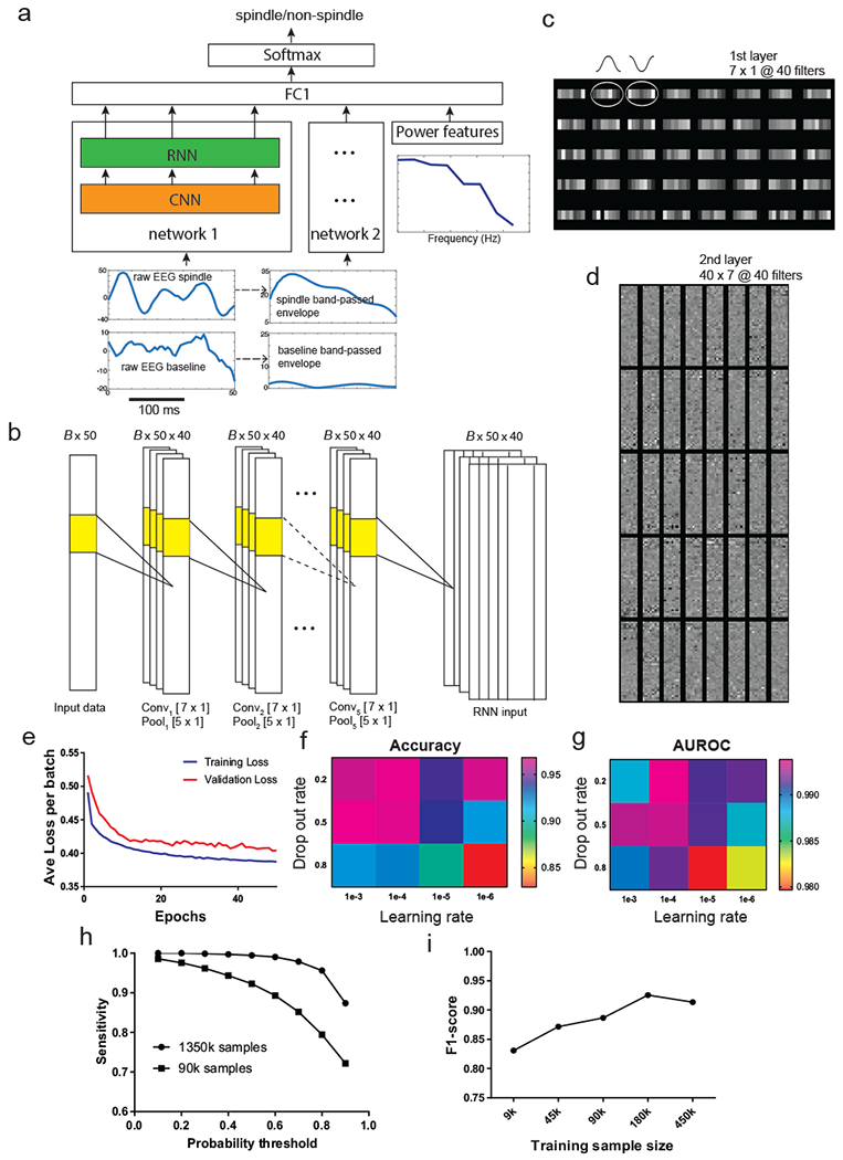
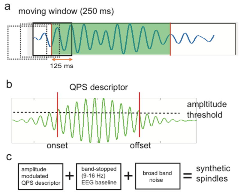
Approach: Here we propose a novel deep learning strategy (SpindleNet) to detect sleep spindles based on a single EEG channel. While the majority of spindle detection methods are used for off-line applications, our method is well suited for online applications.

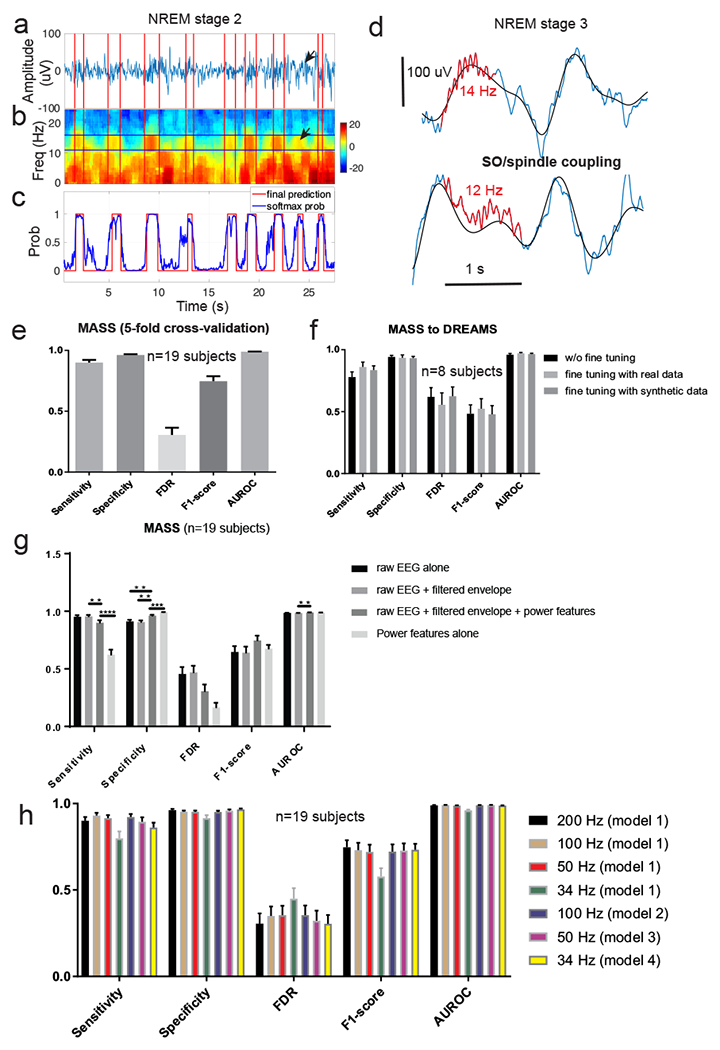
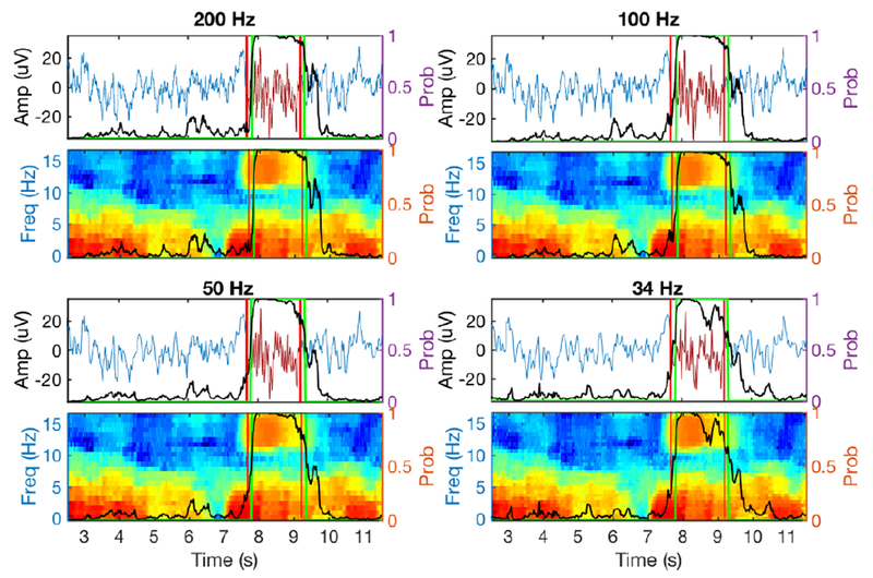
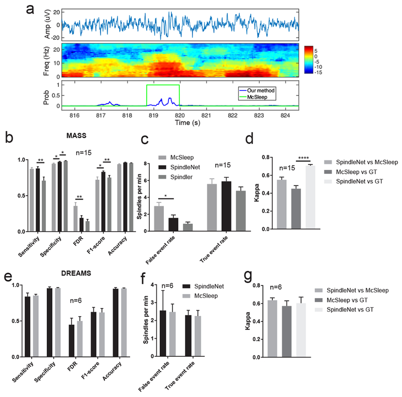
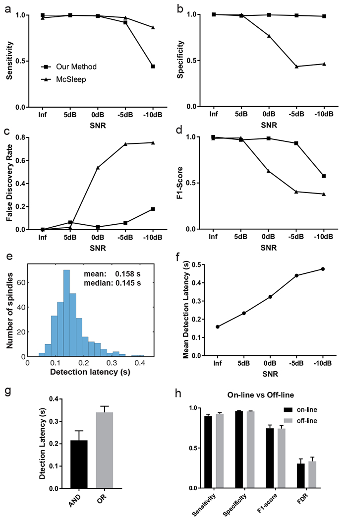
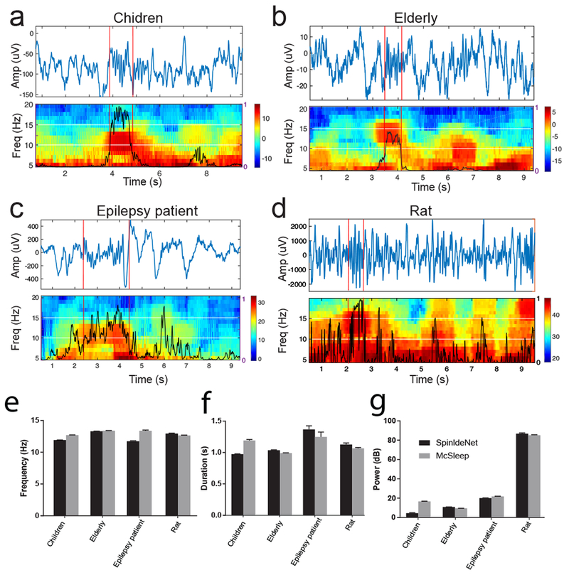
Main results: Compared with other spindle detection methods, SpindleNet achieves superior detection accuracy and speed, as demonstrated in two publicly available expert-validated EEG sleep spindle datasets. Our real-time detection of spindle onset achieves detection latencies of 150-350 ms (~two-three spindle cycles) and retains excellent performance under low EEG sampling frequencies and low signal-to-noise ratios. SpindleNet has good generalization across different sleep datasets from various subject groups of different ages and species.

Significance: SpindleNet is ultra-fast and scalable to multichannel EEG recordings, with an accuracy level comparable to human experts, making it appealing for long-term sleep monitoring and closed-loop neuroscience experiments.

Figure 1.. Statistics of MASS dataset.

a, Statistics of NREM duration (min) on 19 human subjects. b-d, Statistics of annotated spindle number (b), onset time difference between two experts (c) and amplitude standard deviation (d). In panel c, n/a represents the condition only one expert’s annotation was available; the onset time difference among 15 subjects were 0.167 ± 0.007 s (mean±SEM). e-h, In subject #1, statistics discrepancy between two experts on the commonly annotated sleep spindles’ normalized power (e), duration (f), power ratio (g) and difference between two experts (Expert 2-Expert 1) on the spindle onset and duration (h).

Figure 2.. SpindleNet: deep neural network (DNN) architecture used for spindle detection.

a, Overall architecture of the network. The input to subnetwork 1 and 2 consists of raw EEG signal and the envelope of bandpass filtered (9-16 Hz) EEG signal, respectively. The power features that are directly input to the fully connected layer consist of the ratio of the average power of spindle-band frequencies (9-16 Hz) to that of lower frequencies (2-8 Hz) and the instantaneous power of all frequencies from (2-16 Hz). The convolutional neural network (CNN) acts as a temporal feature extractor. The features learned by the CNN are further passed to a recurrent neural network (RNN) that is intendent to discover temporal patterns within the CNN features. The RNN implementation consists of a single-layer long short-term memory (LSTM). The output of the RNN (from 50 time steps) of subnetwork 1 is combined with the output of RNN from the subnetwork 2 and the power features using a fully connected layer. Output of this layer (of length 50) is further processed by a softmax activation function that produces a probability output (spindle vs non-spindle). b, Detailed architecture of the 5-layer CNN. The input is processed by a total of 5 layers. Every layer consists of 40 1D filters of size 7×1, followed by max-pooling with kernel size 5×1. For 250-ms EEG with 200 Hz sampling frequency, the size of input is 50. Batch size is set to B=20. c, A set of 7×1 learned receptive fields (RFs) from the first-layer CNN filters upon completion of training. The 1D filters share a resemblance to the shape of half cycle of spindle oscillation. d, A set of 40×40×7 learned RFs from the second-layer CNN filters. e, The learning convergence curve on training and validation data. f, The change of detection accuracy with respect to two learning hyperparameters: learning rate and drop-out rate. g, The change of AUROC statistic with respect to the learning rate and drop-out rate. h, The sensitivity of spindle detection improved with increasing training sample size (both tested on the same test data). i, The F1-score of detection gradually increased with increasing training sample size.

Figure 3.. Spindle data augmentation and generation of synthetic spindles.

a, We used a 250-ms overlapping moving window (dashed and solid boxes) to construct positive and negative samples. Any EEG traces with ≥50% duration (i.e., 125 ms) coverage of the annotated spindle event (shaded period) was treated as a spindle (positive) example; everything else was a non-spindle (negative) example. b, An amplitude-modulated, quadratic parameter sinusoid (QPS) descriptor for spindles. The two vertical lines mark the onset and offset of spindles, which pass the threshold of 20% of peak amplitude. c, Schematic diagram of generating synthetized sleep spindles.

Figure 4.. Results on online sleep spindle detection.

a, A representative snapshot of EEG trace (during stage-2 NREM sleep) with human marked sleep spindles (in red). b, Associated EEG multi-taper spectrogram (1 s moving window, 5 ms step size). Arrows in panels a and b denote a potentially unlabeled spindle by two experts, which was detected by SpindleNet. c, Softmax probability output (blue) and the final hard decision (red, probability threshold 0.9) for online spindle detection. d, Representative EEG traces (blue) during stage-3 NREM sleep that demonstrate coupling between slow wave (0.5-4 Hz, black trace) and spindles (marked in red). In these two examples, fast (13-16 Hz) sleep spindles tend to occur in the ascending phase of SO cycle (or be coordinated with depolarizing cortical up state), whereas slow (9-12 Hz) spindles tend to occur in the descending phase of SO cycle, or during the transition from cortical down to up states. Note that a large latency in spindle detection may switch from the up ascending phase to the down descending phase of the SO. e, Summarized results (from 5-fold cross validation) of sensitivity, specificity, false discovery rate (FDR), F1-score and AUROC statistics in the MASS dataset (n=19 subjects). Error bar represents SEM. f, Summarized results of sensitivity, specificity, FDR, F1-score and AUROC statistics in the DREAM dataset (n=8 subjects), using SpindleNet trained from the MASS dataset without further fine tuning as well as with fine-tuning using real and simulated spindles. Fine-tuning with real and simulated data further improved the performance. Error bar represents SEM. g, Performance comparison (5-fold cross-validated results) of DNN using different input features: raw EEG signal, filtered EEG envelope within the spindle frequency band (9-16 Hz), and the power feature. h, Results on spindle detection from the MASS dataset (n=19 subjects, error bar represents SEM) under various EEG sampling frequencies. Model 1: standard model trained with EEG signal with 200 Hz sampling rate; Models 2-4: models trained on down-sampled EEG signals at frequencies 100 Hz, 50 Hz, 34 Hz, respectively. In testing EEG signals with <200 Hz sampling frequency, we either up-sampled the signal and applied the standard model (Model 1), or applied the respective model for the sampling frequency. SpindleNet demonstrated robust performance across various sampling frequencies.

Figure 5.. Illustration of EEG traces and spectrograms with annotated (between two red vertical lines) and detected (marked by green vertical lines) sleep spindles at four different sampling frequencies.

Black trace denotes the softmax probability output from SpindleNet. Despite the lower sampling rate and loss of fidelity in EEG spindles, SpindleNet detected the spindle onset reliably.

Figure 6.. Performance comparison between SpindleNet and two other spindle detection algorithms (McSIeep and Spindler).

a, Examples of sleep spindle detection where the McSIeep algorithm detected a false event in the MASS dataset, whereas the softmax probability output (blue trace) from SpindleNet was below the detection threshold. b,c, Summarized comparative performance on the reduced MASS dataset (n=15 subjects, with annotations from two experts). *, p<0.05; **, p<0.01, unpaired t-test. d, Comparison of the kappa statistic between SpindleNet and McSleep, as well as between them and ground truth (GT). e-g, Similar to panels b-d, except for the reduced DREAMS dataset (n=6 subjects, with annotations from two experts).

Figure 7.. Performance comparison between our method (SpindleNet) and McSleep on simulated sleep spindle data with varying levels of signal-to-noise ratio (SNR).

a, Sensitivity. b, Specificity. c, False discovery rate. d, F1-score. The Inf SNR denotes the noiseless condition. e, Histogram of detection latency in the noiseless condition. f, Mean detection latency of our proposed method with respect to the SNR. g, Spindle detection latency based on the AND and OR criteria. Error bar represents SEM (n=19 subjects). h, Performance comparison of on-line vs off-line detection in SpindleNet. Error bar represents SEM (n=19 subjects, MASS dataset).

Figure 8.. Representative examples of sleep spindle detection from various sleep datasets.

a, Children (CHAT). b, Elderly (MrOS). c, Epilepsy patient. d, Rat. e-g, Comparison of detected sleep spindle characteristics (frequency, duration and power) between SpindleNet and the McSleep algorithm.

Figure 9.. Sleep spindle detection performance with respect to different normalization factors.

a, False event rate and true event rate for pre- and post-computed normalization on the MASS dataset (n=19). b, Sensitivity, specificity, FDR, F1-score, accuracy and AUROC for pre- and post-computed normalization on the MASS dataset (n=19). Pre-computed normalization is the average spindle standard deviation from the training set, whereas post-computed normalization is the average standard deviation from the testing set. c, Testing on the MASS subject #18 with various normalization factors in sleep EEG calibration.

References

1. Antoniades Andreas et al. 2017. “Detection of Interictal Discharges With Convolutional Neural Networks Using Discrete Ordered Multichannel Intracranial EEG.” IEEE Transactions on Neural Systems and Rehabilitation Engineering 25(12): 2285–94. - PubMed
1. Antony James W., and Paller Ken A.. 2017. “Using Oscillating Sounds to Manipulate Sleep Spindles.” Sleep 40(3): 1–8. - PMC - PubMed
1. Astori Simone, Wimmer Ralf D., and Anita Lüthi. 2013. “Manipulating Sleep Spindles - Expanding Views on Sleep, Memory, and Disease.” Trends in Neurosciences 36(12): 738–48. - PubMed
1. Babadi Behtash et al. 2012. “DiBa: A Data-Driven Bayesian Algorithm for Sleep Spindle Detection.” IEEE Transactions on Biomedical Engineering 59(2): 483–93. - PubMed
1. Bashivan Pouya, Rish Irina, Yeasin Mohammed, and Codella Noel. 2015. “Learning Representations from EEG with Deep Recurrent-Convolutional Neural Networks.” : 1–15. http://arxiv.org/abs/1511.06448.
Publication types