The modular organization of human anatomical brain networks: Accounting for the cost of wiring

Abstract

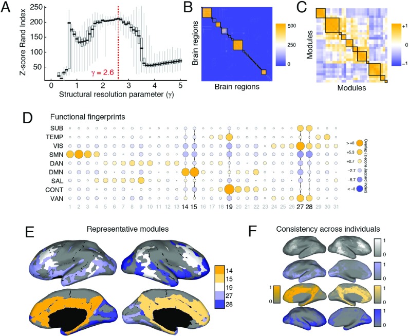
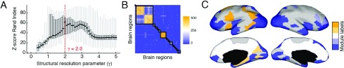
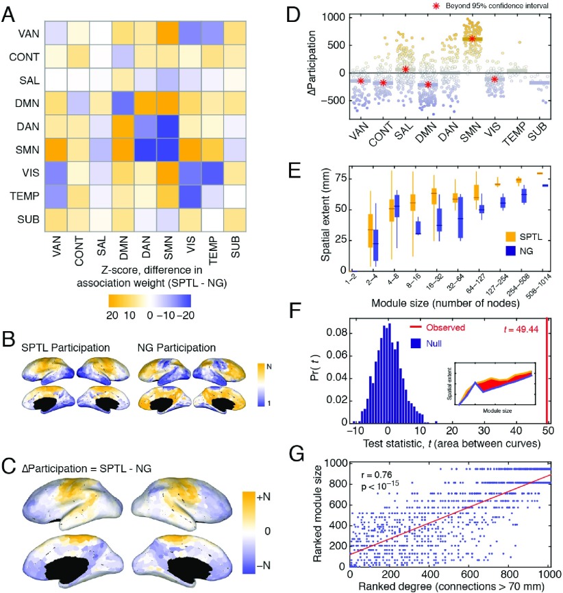
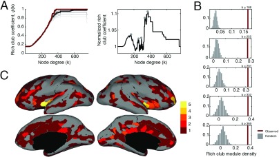
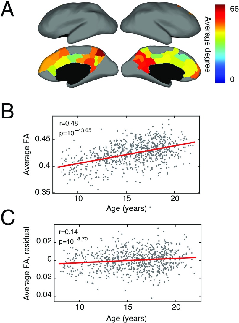
Brain networks are expected to be modular. However, existing techniques for estimating a network's modules make it difficult to assess the influence of organizational principles such as wiring cost reduction on the detected modules. Here we present a modification of an existing module detection algorithm that allowed us to focus on connections that are unexpected under a cost-reduction wiring rule and to identify modules from among these connections. We applied this technique to anatomical brain networks and showed that the modules we detected differ from those detected using the standard technique. We demonstrated that these novel modules are spatially distributed, exhibit unique functional fingerprints, and overlap considerably with rich clubs, giving rise to an alternative and complementary interpretation of the functional roles of specific brain regions. Finally, we demonstrated that, using the modified module detection approach, we can detect modules in a developmental dataset that track normative patterns of maturation. Collectively, these findings support the hypothesis that brain networks are composed of modules and provide additional insight into the function of those modules.

Keywords: Community structure; Complex networks; Geometry; Modularity; Wiring cost.

Figure 1.

Synthetic networks and an illustration of the problem. (A) We show six synthetic networks with the same connection density, three of which are amodular (random, lattice, and geometric); the remaining three have two, four, and eight modules respectively. (B) The modularity function, Q, is greatest for the eight-module network, but the lattice and geometric networks, though formed through fundamentally amodular generative processes, exhibit the next-greatest Q values. This indicates that Q can mistakenly give the impression that networks with no modules are, in fact, highly modular. (C) The majority of connections in anatomical brain networks are short-range and can be accounted for parsimoniously by a cost-reduction mechanism. Our aim is to perform module detection on observed connections that are unanticipated by a cost-reduction mechanism; these connections tend to be long-distance connections, as they are more costly. (D) The result of this refocusing is that, instead of modules whose internal connections are short-range (top), we detect modules linked by long-distance connections (bottom).

Figure 2.

Typical input matrices. (A) Representative connectivity matrix for the DSI dataset. (B) Interregional distance matrix, calculated as the Euclidean distance between the centroids of the N brain regions (nodes). (C) To fit the SPTL model to the observed connectivity matrix, we find the curve through a two-dimensional parameter space (characterized by a density penalty α and a length penalty β ) for which the observed number of connections, M, is equal to the expected number of connections, 〈M〉. Along this curve, we then identify the α *, β * that maximize $\mathcal{L}$, the log-likelihood that the SPTL model generated the observed connectivity network. (D) Fitting the SPTL model returns a matrix whose elements give the probability that any pair of nodes will be connected.

Figure 3.

SPTL modules in human DSI, (A) Distribution of z-score Rand indices as a function of γ . (B) Association matrix (fraction of times out of 500 Louvain runs that each pair of nodes were assigned to the same module) clustered according to consensus modules. The 31 statistically signicant consensus modules exhibited correlated (C) functional fingerprints (D). (E) Here we show the five largest consensus modules on the cortical surface. Each color corresponds to a different module. (F) To demonstrate that these consensus modules, which we uncovered from a representative connectivity matrix, were also expressed at the level of individual subjects, we identified for each subject and for each consensus module, the module with greatest overlap and averaged the nodes that comprised that module to obtain a consistency score. The colorbars show the level of consistency across subjects.

Figure 4.

SPTL modules in human DTI, (A) Distribution of z-score Rand coefficients as a function of γ . (B) Association matrix (fractions of times out of 500 Louvain runs that each pair of nodes were assigned to the same module) clustered according to consensus modules. (C) The five statistically significant consensus modules shown on the cortical surface. Each color corresponds to a different consensus module.

Figure 5.

Comparing properties of SPTL and NG modules, (A) Differences in the SPTL and NG association matrices, grouped by functional systems and z-scored against a null distribution. (B) Ranked node-level participation coefficients on the cortical surface, based on the SPTL (left) and NG (right) modules. (C) Differences between ranked SPTL and NG participation coefficients. (D) System-level changes in participation coefficients. Each point represents a single brain region. The bars represent the median changes in participation coefficients over all regions assigned to each system. A red star indicates that the median change exceeds the 95% confidence interval of the null distribution. (E) The spatial extent (mean interregional distance) of modules, as a function of module size, for both the SPTL and NG models. (F) The area between the two module-size versus spatial-extent curves (inset) serves as a test statistic under functional data analysis (FDA). We compared the observed statistic to the test statistics estimated, had module assignments been random. (G) Correlation of a region’s number of long-distance connections with the size of the module to which it was assigned.

Figure 6.

Results of rich-club analysis. (A) (left) Raw rich-club coefficients (in red) as a function of node degree. The black line represents the mean rich-club coefficient over 1,000 random (degree-preserving) networks. Each increasingly brighter gray line represents one standard deviation away from that mean (up to three standard deviations). (right) The normalized rich-club coefficients (observed raw divided by random mean), which exhibited five local maxima at k = 166,255,291,332,369. (B) Rich-club module density, d_r , for each of the five rich clubs we investigated. In red is the observed value of d_r , while the gray shows the null distribution of densities over 10,000 randomizations. (C) Topographic visualization of rich-club consistency across the cerebral cortex (note: subcortical regions are not pictured). Colored regions indicate how many of the five rich clubs a region participated in, with brighter colors indicating greater participation.

Figure 7.

SPTL modules over development. (A) We observed that a single module exhibited changes in its average internal white-matter integrity (as measured by fractional anisotropy; FA). This module consisted of precuneus, posterior cingulate, and anterior cingulate cortex. The color of each region indicates its degree in the representative connectivity matrix. (B) Without correction for confounding variables, we observed a statistically significant increase in the average within-module FA over development. (C) This relationship, albeit attenuated, persisted after correcting for confounding network, physiological, and morphological variables.

References

1. Ahn Y. Y., Bagrow J. P., & Lehmann S. (2010). Link communities reveal multiscale complexity in networks. Nature, 466(7307), 761– 764. - PubMed
1. Aldecoa R. & Marín I. (2013). Exploring the limits of community detection strategies in complex networks. Scientific Reports, 3, 2216. - PMC - PubMed
1. Andrews-Hanna J. R., Reidler J. S., Sepulcre J., Poulin R., & Buckner R. L. (2010). Functional-anatomic fractionation of the brain’s default network. Neuron, 65(4), 550–562. - PMC - PubMed
1. Arenas A., Fernandez A., & Gomez S. (2008). Analysis of the structure of complex networks at different resolution levels. New Journal of Physics, 10(5), 053039.
1. Avena-Koenigsberger A., Goñi J., Betzel R. F., van den Heuvel M. P., Griffa A., Hagmann P., … Sporns O. (2014). Using Pareto optimality to explore the topology and dynamics of the human connectome. Philosophical Transactions of the Royal Society B, 369(1653), 20130530. - PMC - PubMed
LinkOut - more resources