Model selection may not be a mandatory step for phylogeny reconstruction

Abstract

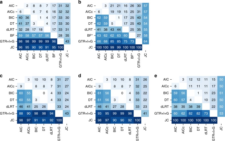
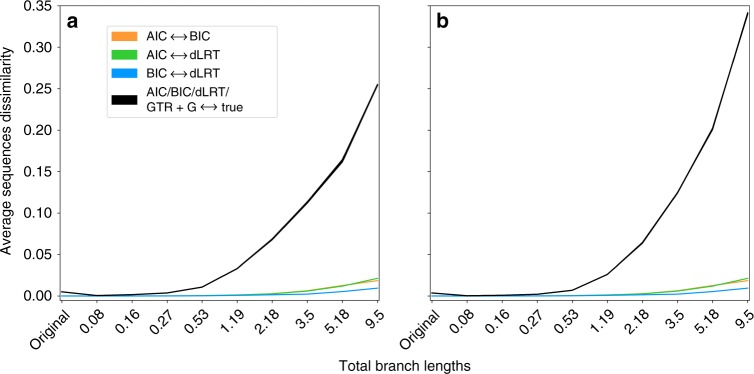
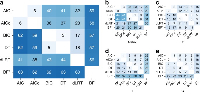
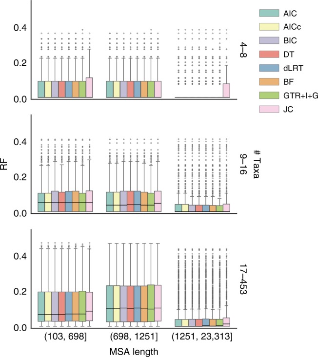
Determining the most suitable model for phylogeny reconstruction constitutes a fundamental step in numerous evolutionary studies. Over the years, various criteria for model selection have been proposed, leading to debate over which criterion is preferable. However, the necessity of this procedure has not been questioned to date. Here, we demonstrate that although incongruency regarding the selected model is frequent over empirical and simulated data, all criteria lead to very similar inferences. When topologies and ancestral sequence reconstruction are the desired output, choosing one criterion over another is not crucial. Moreover, skipping model selection and using instead the most parameter-rich model, GTR+I+G, leads to similar inferences, thus rendering this time-consuming step nonessential, at least under current strategies of model selection.

Fig. 1

Pairwise incongruencies on the trees inferred by the evaluated strategies. The number within each cell represents the percentage of discrepancies between the two strategies at the row and column. The best-fitted model was computed for each criterion, and the trees were reconstructed using ML optimizations according to this model, as well as for the most complex and simplest models—GTR+I+G and JC. For each pair of strategies (rows and columns) the percentage of non-identical trees over 7200 datasets is presented (see * and ** below). The upper right triangles represent the percentages of different topologies and the lower left triangles represent different branch-length estimates. Clearly, two different models lead to different branch-length estimates, hence the latter reflect the percentages of differently selected models. The panels represent the following datasets: a simulation set c₀, b the empirical set, c simulation set c₁, d simulation set c₂, and e simulation set c₃**. (*) The percentages in the row and column of the BF criterion in panel b were computed over a subset of 1500 empirical datasets for which BF was computed (marked with an asterisk; see Methods). The analysis over this subset of 1500 datasets for all comparisons is presented in Supplementary Figure 1. (**) The percentages of the simulation set c₃ were computed over a subset of 1000 datasets that represent coding sequences (see Methods)

Fig. 2

The impact of model selection criteria on ancestral sequence reconstruction. The y axis represents the fraction of sequence sites that were different between every pair of root sequences, averaged across 1000 examined datasets: the black curves (which merge due to negligible differences) represent the comparison between the true root sequence and the inferred one according to the models selected by each of the criteria AIC, BIC, and dLRT, or consistently using GTR+G, and the colored curves represent the differences between every pair of criteria. The results of AICc and DT were similar to AIC and BIC, respectively, thus they are not shown. To increase the variety of sequence divergence, the analysis was repeated for trees that were resized to several scales (x axis). The left and right plots represent the analysis on a simulation set c₀; b complex simulation set c₂. For the numerical estimates, see Supplementary Table 1

Fig. 3

Incongruency over the selection of models for the empirical and simulated datasets. The matrices represent the percentage of the 7200 datasets for which a pair of criteria in the corresponding column and row disagreed on. a represents the disagreement over the entire model (one of 24 models) while (b–e) represent disagreement over components of the models: b the substitution matrix that determines the substitution rates between the nucleotides, such that an equal parameter for all pairs defines JC and F81, two rates for transitions and transversions define K2P and HKY, and an independent parameter for each of the six pairs defines SYM and GTR, c the inclusion of the F component, i.e., equal base frequencies represent JC, K2P, and SYM, whereas unequal frequencies represent F81, HKY, and GTR, d the inclusion of the I parameter (proportion of invariable sites), e the inclusion of the G parameter (heterogeneous rates across sites following the gamma distribution). The percentages below and above the left diagonal represent the percentage of dissimilarities over empirical set and simulation set c₀, respectively. The percentages in the row of the BF criterion are among a subset of 1500 empirical datasets for which BF was computed (marked with an asterisk; see Methods). The analyses over this subset of 1500 datasets for all pairs of criteria is presented in Supplementary Figure 4

Fig. 4

RF distances across different alignment sizes for simulation set c₀. RF distances (y axes) were measured between trees reconstructed according to every strategy (denoted by the different colors) and the corresponding true trees. The data are binned according to the number of taxa (right-vertical axis) and alignment length (horizontal axis). The RF distances are divided by the number of nodes in the trees for a valid comparison across different tree sizes within a bin. The central horizontal lines represent the median values. The bounds of the boxes represent the first and third quartiles (q1 and q3, respectively). The whiskers extend to (q3−q1) × 1.5 beyond the quartiles

References

1. Jukes, T. H. & Cantor, C. R. in Mammalian Protein Metabolism. 21–132 (Academic Press, Cambridge, 1969).
1. Felsenstein J. Evolutionary trees from DNA sequences: a maximum likelihood approach. J. Mol. Evol. 1981;17:368–376. doi: 10.1007/BF01734359. - DOI - PubMed
1. Kimura M. A simple method for estimating evolutionary rates of base substitutions through comparative studies of nucleotide sequences. J. Mol. Evol. 1980;16:111–120. doi: 10.1007/BF01731581. - DOI - PubMed
1. Hasegawa M, Kishino H, Yano Taki. Dating of the human-ape splitting by a molecular clock of mitochondrial DNA. J. Mol. Evol. 1985;22:160–174. doi: 10.1007/BF02101694. - DOI - PubMed
1. Zharkikh A. Estimation of evolutionary distances between nucleotide sequences. J. Mol. Evol. 1994;39:315–329. doi: 10.1007/BF00160155. - DOI - PubMed
Publication types