A Model of Motion Processing in the Visual Cortex Using Neural Field With Asymmetric Hebbian Learning

Abstract

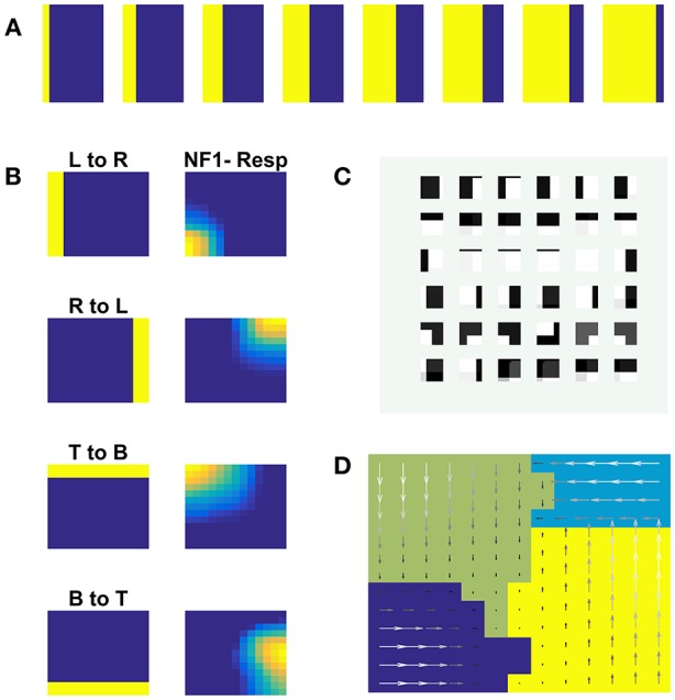
Neurons in the dorsal pathway of the visual cortex are thought to be involved in motion processing. The first site of motion processing is the primary visual cortex (V1), encoding the direction of motion in local receptive fields, with higher order motion processing happening in the middle temporal area (MT). Complex motion properties like optic flow are processed in higher cortical areas of the Medial Superior Temporal area (MST). In this study, a hierarchical neural field network model of motion processing is presented. The model architecture has an input layer followed by either one or cascade of two neural fields (NF): the first of these, NF1, represents V1, while the second, NF2, represents MT. A special feature of the model is that lateral connections used in the neural fields are trained by asymmetric Hebbian learning, imparting to the neural field the ability to process sequential information in motion stimuli. The model was trained using various traditional moving patterns such as bars, squares, gratings, plaids, and random dot stimulus. In the case of bar stimuli, the model had only a single NF, the neurons of which developed a direction map of the moving bar stimuli. Training a network with two NFs on moving square and moving plaids stimuli, we show that, while the neurons in NF1 respond to the direction of the component (such as gratings and edges) motion, the neurons in NF2 (analogous to MT) responding to the direction of the pattern (plaids, square object) motion. In the third study, a network with 2 NFs was simulated using random dot stimuli (RDS) with translational motion, and show that the NF2 neurons can encode the direction of the concurrent dot motion (also called translational flow motion), independent of the dot configuration. This translational RDS flow motion is decoded by a simple perceptron network (a layer above NF2) with an accuracy of 100% on train set and 90% on the test set, thereby demonstrating that the proposed network can generalize to new dot configurations. Also, the response properties of the model on different input stimuli closely resembled many of the known features of the neurons found in electrophysiological studies.

Keywords: lateral interactions; medial superior temporal area (MST); middle temporal area (MT); neural field models; pattern selectivity; primary visual area (V1); weight asymmetry.

Figure 1

The architecture of the motion processing system. (A) Neural field Model: It consists of two NFs, analogous to V1 and MT of the visual cortex. Input layer represents the receptor surface such as the retina. Each NF is organized as a two-dimensional array of neurons with lateral connections. Every neuron has excitatory afferent (incoming; shown in dotted lines) connections from units in their square-shaped RF. Neighboring neurons have overlapping RFs. In addition, every neuron receives inputs from two types of lateral connections: excitatory connections (green circle represents excitatory radius) with nearby neighbors and inhibitory with neurons farther away (red circle represents inhibitory radius). (B) the timeline of input sequence presentation to the network: The model response to a moving stimulus was simulated at two different time scales. The sequence of n frames was presented to the network over a period of time T. Motion within the stimulus sequence was generated at several discrete time steps “t.” The number of time steps is equal to the number of frames within the sequence. For a given time “t” the lateral interactions were allowed to proceed for several time steps “s,” called the settling time.

Figure 2

Direction sensitivity. (A) The Architecture used to simulate the direction sensitivity of V1 cells: The model consists of two stages: (a) an input layer where moving bar is presented (b) NF (20 × 20 units) analogous to V1. Green arcs represent the excitatory connections and the red arcs represent the inhibitory connections. The afferent connections are represented with blue dotted lines (B). Sample bar stimulus moving in 135°: the bar of size 30 × 2 pixels are placed on 64 × 64 pixels black background and is made to move in 8 directions with the direction of motion perpendicular to the orientation. The motion is captured in a sequence of 8 frames. (C) Network response to moving bar stimulus after 500 epochs of training: the first and the third columns display the first frame of the moving bar sequence, the label above it shows the direction of motion of the bar. The response of NF has plotted in the second and fourth columns. Each input is mapped to the unique spatial position on NF. (D) Direction selectivity map: Direction selectivity map is plotted using the convention described in the section “Generating topographic map.” We observed that the patch of neurons selective to one direction of motion often has an adjacent patch with opposite direction preference. The arrows indicate the direction preferences developed by the neurons on NF. The arrow with the highest magnitude indicates the peak response of the neuron (E). The afferent weights developed by the selected neurons in NF: Initial afferent weights are random. After training Gabor like afferent weights are developed. Different varieties of tuned afferent weights (64 × 64 pixels each) are selected from the whole population (Figure S1) and displayed here.

Figure 3

Aperture Problem. (A) A grating pattern consisting of alternating black and white bars. The grating is allowed to move in different directions. Thin arrows in (A) represent the set of physical motions of the grating pattern in various directions. The motion of all these grating patterns is indifferent when viewed through a small window, and this motion direction is perpendicular to the orientation of the grating (as a thick arrow shown in B). This ambiguity in determining the direction of motion of the grating is termed as aperture problem. In case of motion of a two-dimensional object (e.g., square or diamond), local motion cues (dotted arrows show in C) are divergent and are very different from the actual object motion. In (D) thin arrows represent the local motion of each edge seen through RF. An intersection of two constraint lines from both the edges represents the true motion of an object (thick arrow in D).

Figure 4

NF1 neuron preferences to moving edge stimuli. NF1 of the two-NFs network is trained using moving square stimuli. 24 × 24 pixel white square is moved on 64 × 64 pixel black background. As neurons in NF1 has small receptive fields (12 × 12 pixels), at any instance, it can see a part of a square and become selective to local motion cues also called component motion which is an edge motion in this case. (A) Sample input of an edge (64 × 64 pixels) moving from left to right. An edge can be moved in four possible directions [left to right (L to R), right to left (R to L), top to bottom (T to B) and bottom to top (B to T)] and the response of NF1 to an edge motion is displayed in (B). Even though NF1 is trained using moving square objects, most of the NF1 neurons tuned to local edge motion (i.e., component motion). (C) Depicts the trained afferent weights (12 × 12 pixel each) for the selected neurons. (D) Topographic map formed out of NF1 response to edge motion: The arrows indicate the neuron preferences in the direction of edge motion.

Figure 5

NF2 response to moving Square stimuli. (A–D) are four clusters. In each cluster first column depicts the frames of moving squares stimuli (64 × 64 pixels), and the corresponding activity on NF1 (13 × 13 units), and NF2 (15 × 15 units) are shown in the next two columns. The label on the first column represents the direction of motion of a square object (A: 180°, B: 45°, C: 0°, and D: 225°). Neurons in NF1 respond to local motion cues. At each frame presentation, different neurons receive afferent input from the square object and become active, according to its preferred direction of motion, thus the activity pattern follows the square stimulus. In NF2 neurons are selective to the entire object motion (also called pattern motion) by aggregating local motion cues from NF1. Nearly stabilized activity can be seen over the presentation of the whole moving square sequence. Different patches of neurons uniquely become selective to different directions of square motion. (E) Shows the pattern selectivity map plotted out of NF2 neuron responses to moving square stimuli. The arrows indicate the neuron preferences to 8 motion directions: 0, 45, 90, 135, 180, 225, 270, and 315°. The magnitude of the arrow represents the activity of the neuron. Peak activity is represented by neurons with the highest magnitude. (F) Represents the NF2 afferent weights (13 × 13 pixels each) of the selected neurons. It shows that the NF2 neurons developed spatiotemporal receptive fields in the direction of pattern motion.

Figure 6

NF1 response to moving grating stimuli. Grating stimulus consists of alternating black and white bars. Gratings (64 × 64 pixels) are moved in 8 different directions such that the direction of motion is orthogonal to the grating orientation. Plaid stimulus moving in 0° is created by superimposing two gratings moving in 45° and 135° as shown in (A). NF1 (20 × 20 units) is trained with moving grating stimuli for 1,500 epochs and the response is plotted as shown in (B). Here the first and third columns display the frames of moving grating. The label above it indicates the direction of motion of the grating. The second and the fourth columns represent the neuronal preferences to a given grating. As seen in other simulations, different neuron patches become active to different motion directions. Also, component selectivity map is shown in (C). The arrows indicate the neuron preferred directions of motion.

Figure 7

Two-NFs network response to moving plaid stimuli. the Plaid (64 × 64 pixels) stimulus is created from its components (two gratings) and is allowed to move in 8 different directions. NF1 (analogous to V1) is trained with plaid components (i.e., moving gratings) and its response to moving plaid stimuli is plotted in (A). First, third, fifth, and seventh columns display a frame in moving plaid sequence. The label above it indicates the direction of motion of a plaid. Second, fourth, sixth, and eighth columns represent the NF1 response to plaids, and two neuron populations are active in response to every moving plaid stimulus. As each plaid is composed of two gratings, neurons that are preferential to these moving gratings are becoming active. For example, the plaid moving in 315° is made from gratings moving in 270 and 0°. The activity pattern of these two plaid components (shown in Figure 6B) gets integrated and produces a plaid response as two activity bubbles. NF2 (analogous to MT) is trained using plaid pattern moving in 8 directions, by keeping NF1 weights constant. The response of NF2 to four sample stimuli is shown in (B). The first column represents frames of moving plaid stimuli, second and third columns labeled as NF1-Resp (20 × 20 units) and NF2-Resp (13 × 13 units) represents the responses of NF1 and NF2, respectively. We observed that in response to 8 moving plaid stimuli 8 different patches of neurons become selective to different directions of motion, and the corresponding pattern selectivity map is shown in (C).

Figure 8

NF2 response to translational random dot stimuli. (A) Proposed 2NFs network: both NFs are trained using unsupervised asymmetric Hebbian rule and the third single layer perceptron is trained using backpropagation. Random dots stimulus (RDS) is created by placing tiny squares of size 2 × 2 pixel (assumed as dots) on 32 × 32 pixel size grid randomly with a constraint that each 8 × 8 pixel grid can accommodate only one dot. Thus, 16 dots are placed randomly and moved dots coherently in 4 directions: 0, 90, 180, 270° to create translational flow sequences. Thus, each dot configuration creates 4 sequences for the train set. First, third and fifth columns in (B) shows three different dot configurations moving in the same direction. Second, fourth and sixth columns show the NF2 activity, when these configurations moved in 4 directions. Here the neurons encode the coherent motion direction, independent of the precise dot configuration. (C) It represents the translational flow selectivity map in response to the train set consisting of 80 sequences. The arrow direction indicates the neurons preferred direction of motion to the translational flow stimuli. (D) Error plot obtained while training single layer perceptron using NF2 responses of the train set. Single layer perceptron has an input layer and an output layer; the weights (all-to-all connections) between them are trained using regular backpropagation. Perceptron took nearly 300 epochs to learn the input.

Figure 9

Error graphs obtained during the perceptron training. (A–C) Represents the error plots obtained for Bar, Square, and Plaids respectively, during the perceptron training. The NF layer encodes the motion information of moving stimuli as a unique neuronal population response over a network space. Perceptron takes this population values as input and learns the pattern in the input. The complexity of this response pattern is low to the bar and high to the plaids. The perceptron trained on less complex bar input converges with smooth error graph and the fluctuations were seen in the error graphs of the other two which were proportional to the complexity of the input.

Figure 10

Robustness of the trained network: NF1(20 × 20 units) trained using non-noisy moving bar is used to test the robustness of the proposed network. (A,B) represents the decrease in the robustness index (RI)of the network with an increase in the noise density. The thick black lines in (A,B) indicates the RI average across 20 trials. In the case of salt and pepper noise, RI reaches zero when 50% of the training set pixels were made noisy. Similar results can be seen with Gaussian noise with variance = 1. The network shows high tolerance: to the Gaussian noise with a variance of <0.5 and to the salt and pepper noise whose density of <0.3. (C,D) represents the number of pixels deviated from its preferred direction in relation to the noise density. (E) represents the robustness of the network to the varying bar length. RI reduced slightly with a change in the bar length. (F) shows the number of neurons deviated from their preferred directions to the change in bar length.

References

1. Adelson E. H., Bergen J. R. (1985). Spatiotemporal energy models for the perception of motion. J. Optical Soc. Am. A 2:284. 10.1364/JOSAA.2.000284 - DOI - PubMed
1. Adelson E. H., Movshon J. A. (1982). Phenomenal coherence of moving visual patterns. Nature 300, 523–525. 10.1038/300523a0 - DOI - PubMed
1. Albright T. D. (1984). Direction and orientation selectivity of neurons in visual area MT of the macaque. J. Neurophysiol. 52, 1106–1130. 10.1152/jn.1984.52.6.1106 - DOI - PubMed
1. Bichler O., Querlioz D., Thorpe S. J., Bourgoin J.-P., Gamrat C. (2012). Extraction of temporally correlated features from dynamic vision sensors with spike-timing-dependent plasticity. Neural Networks 32, 339–348. 10.1016/j.neunet.2012.02.022 - DOI - PubMed
1. Blasdel G. (1992). Orientation selectivity, preference, and continuity in monkey striate cortex. J. Neurosci. 12, 3139–3161. 10.1523/JNEUROSCI.12-08-03139.1992 - DOI - PMC - PubMed