Burst Firing and Spatial Coding in Subicular Principal Cells

Abstract

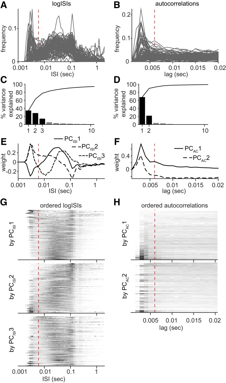
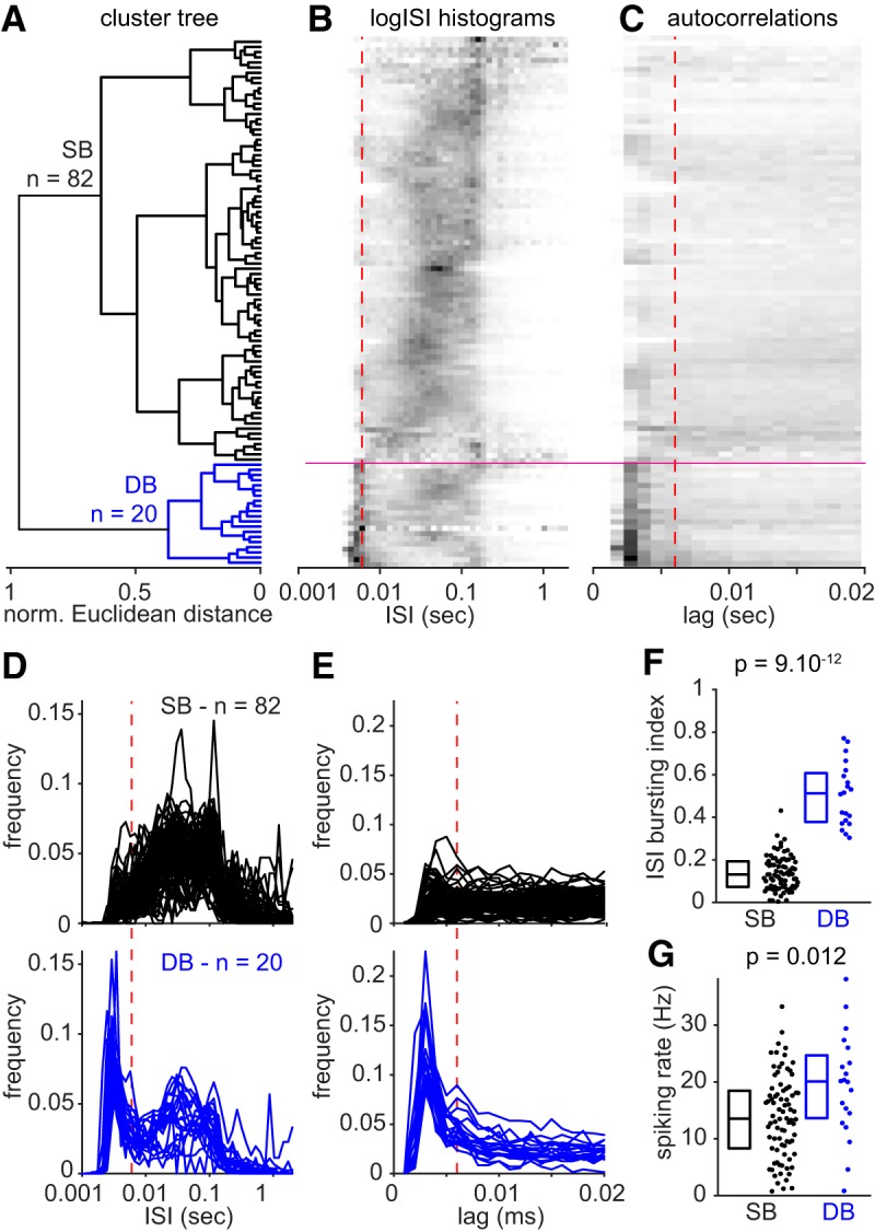
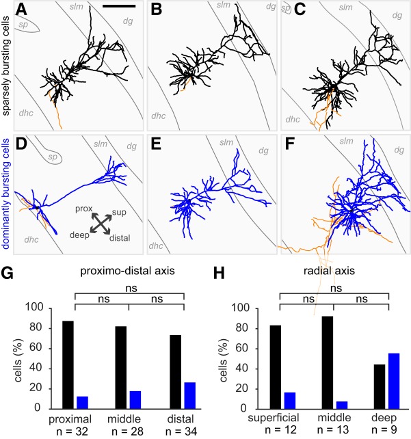
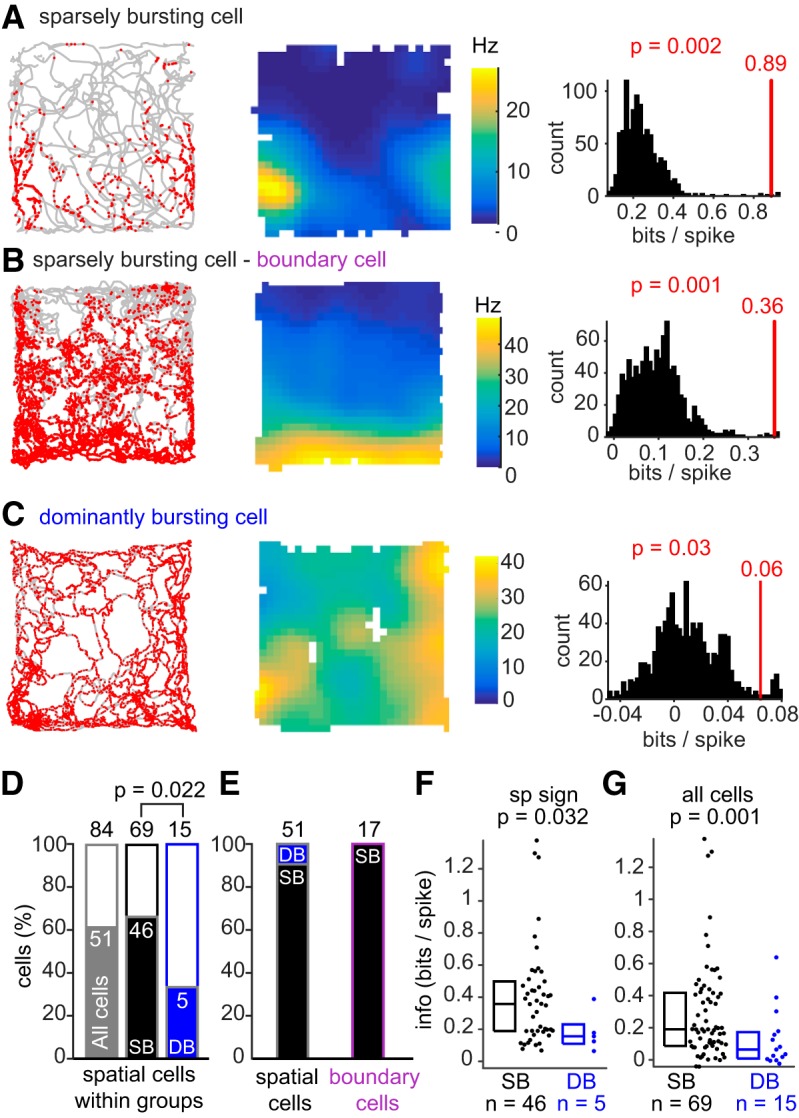
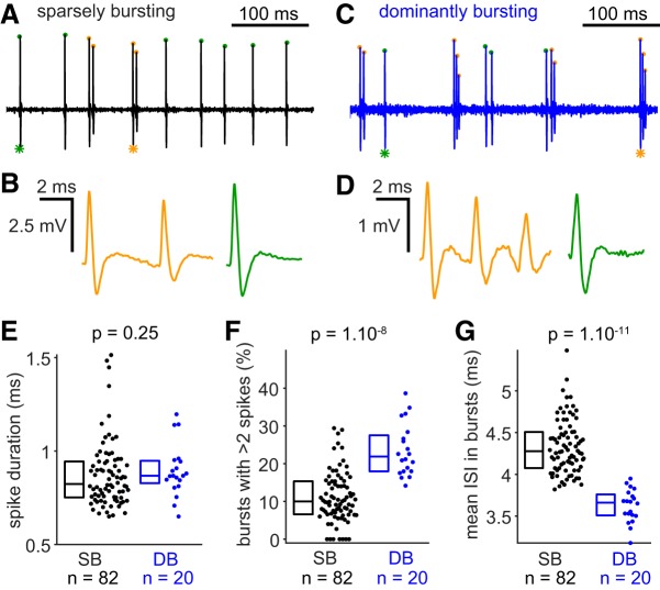
The subiculum is the major output structure of the hippocampal formation and is involved in learning and memory as well as in spatial navigation. Little is known about how neuronal diversity contributes to function in the subiculum. Previously, in vitro studies have identified distinct bursting patterns in the subiculum. Here, we asked how burst firing is related to spatial coding in vivo Using juxtacellular recordings in freely moving male rats, we studied the bursting behavior of 102 subicular principal neurons and distinguished two populations: sparsely bursting (∼80%) and dominantly bursting neurons (∼20%). These bursting behaviors were not linked to anatomy: both cell types were found all along the proximodistal and radial axes of the subiculum and all identified cells were pyramidal neurons. However, the distinct burst firing patterns were related to functional differences: the activity of sparsely bursting cells showed a stronger spatial modulation than the activity of dominantly bursting neurons. In addition, all cells classified as boundary cells were sparsely bursting cells. In most sparsely bursting cells, bursts defined sharper firing fields and carried more spatial information than isolated spikes. We conclude that burst firing is functionally relevant to subicular spatially tuned neurons, possibly by serving as a mechanism to transmit spatial information to downstream structures.SIGNIFICANCE STATEMENT The subiculum is the major output structure of the hippocampal formation and is involved in spatial navigation. In vitro, subicular cells can be distinguished by their ability to initiate bursts as brief sequences of spikes fired at high frequencies. Little is known about the relationship between cellular diversity and spatial coding in the subiculum. We performed high-resolution juxtacellular recordings in freely moving rats and found that bursting behavior predicts functional differences between subicular neurons. Specifically, sparsely bursting cells have lower firing rates and carry more spatial information than dominantly bursting cells. Additionally, bursts fired by sparsely bursting cells encoded spatial information better than isolated spikes, indicating that bursts act as a unit of information dedicated to spatial coding.

Keywords: border cell; cluster analysis; hippocampus; multiplexing; orientation.

Figure 1.

Principal component analyses of ISI distributions and spike autocorrelations during navigation. A, Top, Histogram of the logISI for all subicular principal cells (n = 102). The values of the x-axis have been replaced by the corresponding interval values in seconds. B, Top, Spike autocorrelation for all subicular principal cells (n = 102). The plot is normalized so the 0 ms-lag value is equal to 1 (out of the axis range here). The vertical dashed line is placed at 6 ms. Only navigating periods have been considered for these analyses (rat's speed >3 cm/s). C, Percentage of variance explained by the 10 first principal components of logISI histogram. PC_ISI1, PC_ISI2 and PC_ISI3 explain, respectively, 35, 29, and 15% of the total variance, so approximately 78% in total. D, Percentage of variance explained by the 10 first principal components of spike autocorrelations. PC_AC1 and PC_AC2 explain, respectively, 68 and 22% of the total variance, so 90% in total. E, Loading of the logISI bins into the first three principal components (PC_ISI1, PC_ISI2 and PC_ISI3) of the logISI histogram matrix. The vertical dashed line is placed at 6 ms corresponding to our threshold for burst firing. The short intervals (<6 ms) are similarly loaded in the first three components in contrast with the more delayed intervals. F, The autocorrelation lags are loaded according to similar patterns into the first two principal components (PC_AC1, and PC_AC2). G, The logISI histogram frequency matrix has been ordered according to values on PC_ISI1, PC_ISI2, and PC_ISI3, and plotted in grayscale. One line is one cell; dark values correspond to high frequencies and light values to low frequencies. Cells with an initial peak tend to be distributed on one side (top or bottom), but not clearly grouped together. For each plot, a structure emerges in the delayed ISI range. Using the three first principal components of the logISI frequency matrix seems biologically relevant because they all depict both bursting and other discharge patterns, such as firing rates or theta modulation (peak ∼0.1 s). H, The spike autocorrelation frequency matrix has been ordered according to values on PC_AC1and PC_AC2, and plotted in grayscale. One line is one cell; dark values correspond to high frequencies and light values to low frequencies. PC_AC1 is clearly a good parameter to classify cells according to burstiness as cells with an initial peak (<6 ms) are grouped together at the bottom of the color plot. PC_AC2 is not as good for predicting bursting behavior, even though a few cells with an initial peak can be found again at the bottom of the color plot.

Figure 2.

Classification of subicular principal cells based on their firing patterns during navigation. A, Hierarchical cluster tree of subicular principal cells based on the logISI and spike autocorrelation principal component analyses. The Ward's method, an agglomerative hierarchical clustering procedure was used to generate the cluster tree based on normalized Euclidean distance between cells in a 5-dimensional space, defined by PC_ISI1, PC_ISI2, PC_ISI3, PC_AC1, and PC_AC 2. The black branch corresponds to SBs and the blue branch corresponds to DBs. B, C, logISI histogram and spike autocorrelation frequency matrices have been ordered as on the cluster tree in A and are represented in grayscale plots (black, high values; white, low values). The vertical dashed red lines are positioned at 6 ms. Horizontal magenta lines show the cluster separation on the color plots. Cells with a prominent initial peak in logISI histogram and spike autocorrelation are grouped at the bottom of the representations and correspond to dominantly bursting cells. D, logISI histograms for SBs (n = 82; top) and DBs (n = 20; bottom). Note the prominent initial peak for dominantly bursting cells, absent for sparsely bursting cells, which highlights a higher proportion of low intervals corresponding to prominent burst firing. E, Spike autocorrelations for sparsely bursting cells (n = 82, top) and dominantly bursting cells (n = 20, bottom). As for the logISI histogram, note the prominent initial peak for dominantly bursting cells, absent for sparsely bursting cells. F, ISI-based bursting index corresponding to the proportion of ISIs <6 ms is significantly higher for dominantly bursting cells. G, Spiking rate (Hz) is significantly higher for dominantly bursting cells. Statistics: two-tailed Mann–Whitney U test; box plots showing median and interquartile ranges.

Figure 4.

A–F, Reconstructions of 6 subicular principal cells. Dendrites are in black (sparsely bursting cells) or blue (dominantly bursting cells) and axons are in orange. Some of the anatomical outlines have been drawn, such as CA1 stratum pyramidale (sp), the stratum lacunosum moleculare (slm) and the limit of the subiculum with the dorsal hippocampal commissure (dhc). dg: dendate gyrus. All cells are oriented as indicated in panel D; prox: proximal; dist: distal; sup: superficial. In A, scale bar = 200 μm. G, Distribution of sparsely bursting and dominantly bursting cells along the proximo-distal axis of the subiculum. Fisher's exact tests, with level of significance corrected to be equal 0.05 in total: ns: p > 0.05/3; proximal vs middle, p = .7211; middle vs distal = 0.5457; superficial vs distal = 0.2183. H, Distribution of sparsely bursting and dominantly bursting cells along the radial axis of the subiculum. Fisher's exact tests (ns: p > 0.05/3); superficial versus middle, p = 0.593; middle versus deep = 0.0231; superficial versus deep = 0.1588.

Figure 5.

Sparsely bursting cells provide more spatial information than dominantly bursting cells. A–C, Left, Trajectories of rat in gray with superimposed spikes in red. Middle, Corresponding rate maps with their color-map ranging from 0 to the maximum firing rate of the cells (Hz). Right, Cell-by-cell spatial significance analyses. Each cell's spatial information (red vertical line) was ranked within the distribution of spatial information values determined using a cell-by-cell circular shuffling procedure (black histogram, see Materials and Methods). For each cell, spatial information was declared significant if the cell's information exceeded the 95th percentile of the random distribution obtained after circular shuffling (see Materials and Methods). All the cells shown in A–C are spatially significant (p < 0.05; see Materials and Methods). Neurons in A and B are sparsely bursting cells; the neuron in C is a dominantly bursting cell. The neuron in B was categorized as a boundary cell (boundary score = 0.73, p = 0.01; see Materials and Methods). D, Spatial information and significance were calculated for subicular cells recorded while the animal explored (speed >3 cm/s) at least 60% of the open-field arena (n = 84/102). The bar graph shows the percentage of spatially modulated cells from all subicular cells (n = 51/84; gray), and then from sparsely bursting cells (n = 46/69; black) and dominantly bursting cells (5/15 cells; blue). Sparsely bursting cells are more often spatially modulated than dominantly bursting cells (p = 0.022: significant Fisher's exact test). E, Percentage of each cell type within spatial cell categories. Left, Sparsely bursting cells represent the majority (n = 46/51) of subicular spatial units. Right, All boundary cells were sparsely bursting cells F, Spatial information calculated for spatially significant sparsely bursting and dominantly bursting cells (p = 0.032, bootstrapping, significant) G, Spatial information calculated for all sparsely bursting cells and dominantly bursting cells (p = 0.001, bootstrapping, significant).

Figure 3.

Spike and burst features of sparsely bursting cells and dominantly bursting cells. A, Bandpass filtered (300–6000 Hz) trace of recording from a sparsely bursting cell. Spikes occurring in bursts are labeled with orange dots and isolated spikes with green dots. B, Magnification of the burst (orange, left) and the isolated spike (green, right) indicated with a star. A and B have the same vertical scale. C, Same as A for a dominantly bursting cell. D, Same as B for a dominantly bursting cell. C and D have the same vertical scale. A and C, as well as B and D have the same horizontal scale. E, Spike duration, from threshold to afterhyperpolarization, is not different between sparsely bursting and dominantly bursting cells. F, Bursts of dominantly bursting cells have more spikes than bursts fired by sparsely bursting cells. G, The mean ISIs inside bursts are shorter in dominantly bursting cells compared with sparsely bursting cells. Statistics: two-tailed Mann–Whitney U test; box plots showing median and interquartile ranges.

Figure 6.

Sharp spatial tuning of burst firing in spatially modulated sparsely bursting cells. A–F, Example plots of sparsely bursting spatial neurons. Spikes, Spikes (red dots) superimposed onto the animal's trajectory (gray line). Isolated spikes, Isolated spikes (green dots) superimposed onto the animal's trajectory (gray line) and corresponding rate map; corrected spatial information below. Bursts, Bursts (orange dots) on animals' trajectories (gray line) and corresponding burst rate maps; spatial information below. Each color-map ranges from 0 to the rate map maximum rate (Hz). Significance, Results of the bootstrapping used to determine significance of burst spatial information compared with isolated spike information. The orange line represents spatial information calculated from the N bursts fired by each cell and the green histogram shows the distribution of spatial information calculated from 1000 random samples of N isolated spikes. Cells in C–F are boundary cells. G, Fraction of cells where burst spatial information is significantly higher than isolated spike spatial information. Within groups, Proportion of all spatial cells, sparsely bursting spatial cells and dominantly bursting spatial cells with a significant difference. From groups, Proportion sparsely bursting cells and dominantly bursting cells in cells showing a significant difference. Boundary cells, Proportion of boundary cells with a significant difference. H, Information per burst versus information per isolated spike for spatially modulated neurons (n = 46 sparsely bursting cells, black circles and purple circles corresponding to boundary cells; n = 5 dominantly bursting cells, blue circle). Solid circles indicate cells with a significant increase of spatial information between bursts and isolated spikes (n = 31/46 for sparsely bursting cells including n = 12/17 boundary cells and n = 3/5 for dominantly bursting cells). I, Spatial information per isolated spike and bursts only for spatial cells with a significant difference, with sparsely bursting cells in black and dominantly bursting cells in blue and boundary cells in purple. Corrected info, Spatial information calculated using similar numbers of bursts and isolated spikes (from the bootstrapping).

References

1. Amaral DG, Witter MP (1989) The three-dimensional organization of the hippocampal formation: a review of anatomical data. Neuroscience 31:571–591. 10.1016/0306-4522(89)90424-7 - DOI - PubMed
1. Barry C, Lever C, Hayman R, Hartley T, Burton S, O'Keefe J, Jeffery K, Burgess N (2006) The boundary vector cell model of place cell firing and spatial memory. Rev Neurosci 17:71–97. 10.1515/REVNEURO.2006.17.1-2.71 - DOI - PMC - PubMed
1. Behr J, Empson RM, Schmitz D, Gloveli T, Heinemann U (1996) Electrophysiological properties of rat subicular neurons in vitro. Neurosci Lett 220:41–44. 10.1016/S0304-3940(96)13242-0 - DOI - PubMed
1. Bjerknes TL, Moser EI, Moser MB (2014) Representation of geometric borders in the developing rat. Neuron 82:71–78. 10.1016/j.neuron.2014.02.014 - DOI - PubMed
1. Böhm C, Peng Y, Maier N, Winterer J, Poulet JF, Geiger JR, Schmitz D (2015) Functional diversity of subicular principal cells during hippocampal ripples. J Neurosci 35:13608–13618. 10.1523/JNEUROSCI.5034-14.2015 - DOI - PMC - PubMed
Publication types
LinkOut - more resources