Control of a Humanoid NAO Robot by an Adaptive Bioinspired Cerebellar Module in 3D Motion Tasks

Abstract

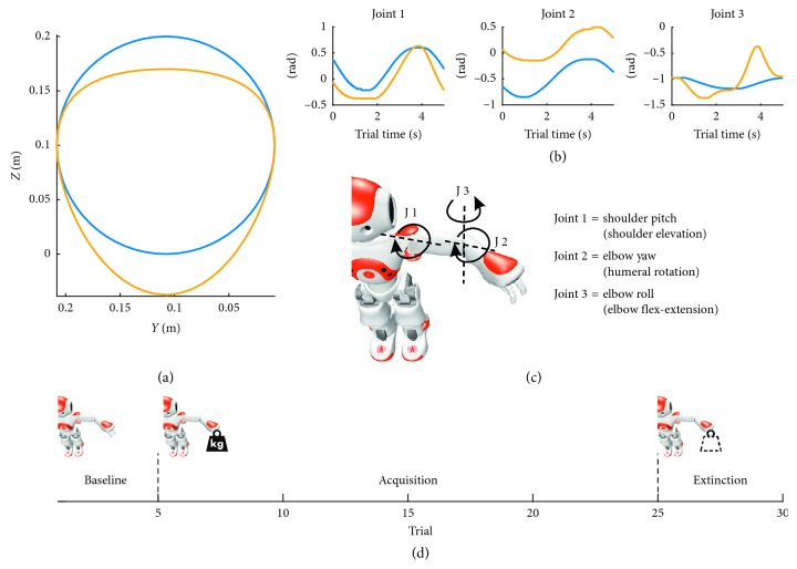
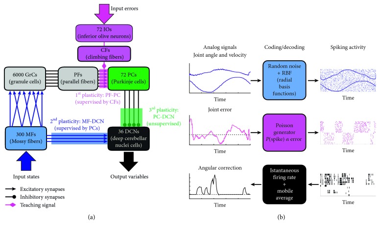
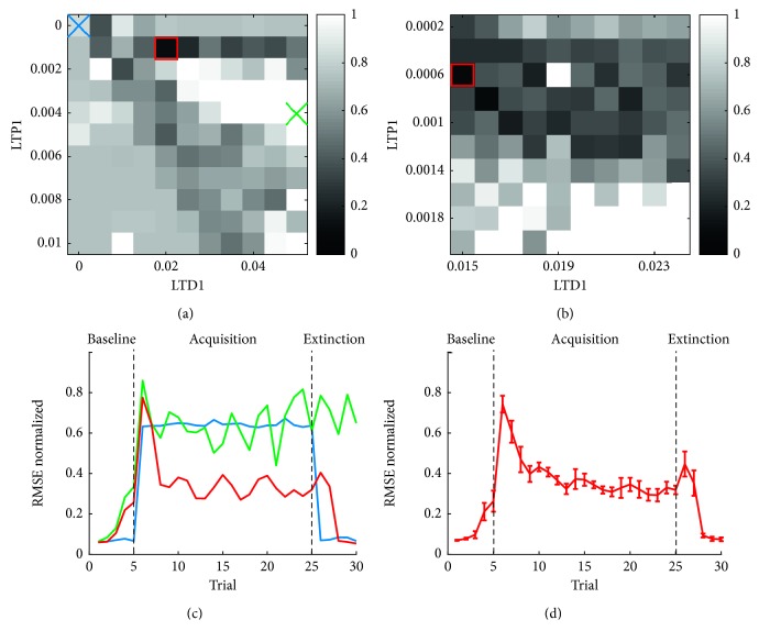
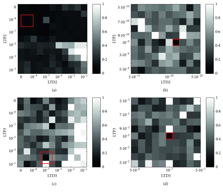
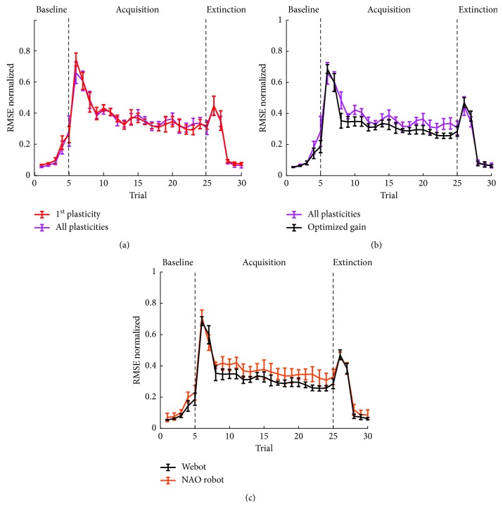
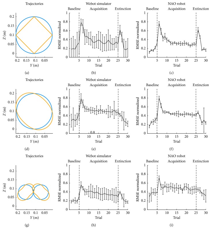
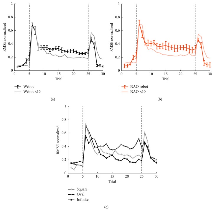
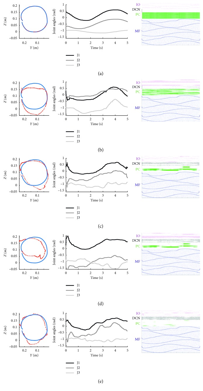
A bioinspired adaptive model, developed by means of a spiking neural network made of thousands of artificial neurons, has been leveraged to control a humanoid NAO robot in real time. The learning properties of the system have been challenged in a classic cerebellum-driven paradigm, a perturbed upper limb reaching protocol. The neurophysiological principles used to develop the model succeeded in driving an adaptive motor control protocol with baseline, acquisition, and extinction phases. The spiking neural network model showed learning behaviours similar to the ones experimentally measured with human subjects in the same task in the acquisition phase, while resorted to other strategies in the extinction phase. The model processed in real-time external inputs, encoded as spikes, and the generated spiking activity of its output neurons was decoded, in order to provide the proper correction on the motor actuators. Three bidirectional long-term plasticity rules have been embedded for different connections and with different time scales. The plasticities shaped the firing activity of the output layer neurons of the network. In the perturbed upper limb reaching protocol, the neurorobot successfully learned how to compensate for the external perturbation generating an appropriate correction. Therefore, the spiking cerebellar model was able to reproduce in the robotic platform how biological systems deal with external sources of error, in both ideal and real (noisy) environments.

Figure 1

Trajectories and experimental protocol. (a) Planar representation (Y-Z axis, in the robot reference frame) of the ideal (blue) and perturbed (yellow) Cartesian trajectories. The corresponding trajectories in the joint space are depicted in panel (b). (c) The controlled joints of the robot correspond to three rotations: shoulder elevation (Joint 1), humeral rotation (Joint 2), and elbow flex extension (Joint 3). (d) The experimental protocol consists of 5 baseline trials, 20 trials of acquisition, where a load is applied to the robot arm, and 5 trials of extinction, where the additional load is removed.

Figure 2

Cerebellar SNN and coding/decoding strategies. (a) The computational model applied for creating the cerebellar SNN embedded into the controller of NAO robot. Each block represents a neural population, with the relative inputs and outputs. The excitatory, inhibitory, and teaching connections are depicted. The shaded areas represent the three plasticity sites: magenta the PF-PC synapses, blue the MF-DCN synapses, and green the PC-DCN synapses, adapted from [15]. (b) Coding (for MFs and IOs) and decoding (for DCNs) strategies implemented to integrate the analog robotic world with the spiking activity of the SNN. The 3 joint angles and angular velocities are fed as input to the MFs by means of an RBF approach, overlapped to a random activity. Each joint error is transformed into IO spikes by means of Poisson generators, which produce spikes with a probability that is proportional to the error magnitude. Each IO generates a spike pattern that is therefore independent of their history and of the other IOs. The DCN spikes are transformed into an angular correction sent to the robot joints by means of an instantaneous firing rate computation, subsequently averaged with a mobile-window filter.

Figure 3

Cortical plasticity optimization. (a) Cost function resulting from the gross exploration of LTP1 and LTD1 parameters. Darkest values represent low values of the cost function, therefore the best combinations of the two plasticity parameters. The parameter space further explored in the finer search (b) is identified by the red square. Blue and green crosses identify two examples parameters giving bad performances (c). (b) Cost function resulting from the finer exploration of LTP1 and LTD1 parameters. The red square identifies the global minimum, therefore the chosen combination of LTP1 and LTD1. (c) Three examples of RMSE performance across the 30 trials of the protocol. The red line represents a good performance, with a reduction of the RMSE during the acquisition phase and a good extinction in the last 5 trials. The blue line represents the combination of LTP1=0.0 and LTD1=0.0; therefore, no correction happened in the acquisition phase, leading to a high cost function value. The green line represents a combination of too high LTP1 and LTD1, leading to an unstable and ineffective correction along the trials. (d) Mean and SD of the RMSE in 10 tests performed with the Webot simulator with the best combination of LTP1 and LTD1 identified in the finer exploration.

Figure 4

Nuclear plasticities optimization. (a, b) Cost functions resulting from the gross and finer explorations of LTP2 and LTD2 parameters. Darkest values represent low values of the cost function, therefore the best combinations of the two plasticity parameters. The parameter space further explored in the finer search (b) is identified by the red square (a). (c, d) As (a, b), but for the gross and finer exploration of LTP3 and LTD3.

Figure 5

RMSE in different testing conditions. (a) Mean and SD of the RMSE computed for 10 tests with only the cortical plasticity optimized (in red) and after the optimization of the cortical and nuclear plasticities (in magenta). (b) Mean and SD of the RMSE computed for 10 tests after the optimization of the cortical and nuclear plasticities (in magenta) and after the optimization of the gain (in black). (c) Mean and SD of the RMSE computed for 10 tests after the optimization of the gain with Webot simulator (in black) and with NAO robot (in orange).

Figure 6

Transfer learning performances. (a, d, g) Ideal (blue) and perturbed (yellow) Cartesian trajectories in three cases: square, oval, and infinite, respectively. (b, e, h) Mean and SD of the RMSE computed for 10 tests with Webot simulator for the respective trajectories. (c, f, i) Mean and SD of the RMSE computed for 10 tests with NAO robot for the respective trajectories.

Figure 7

RMSE with the enhanced SNN. (a) Mean and SD of the RMSE computed for 10 tests with Webot simulator with the standard network (in black) and a single test with the enhanced tenfold SNN (in grey). (b) Mean and SD of the RMSE computed for 10 tests with NAO robot with the standard network (in orange) and a single test with the enhanced tenfold SNN (in light orange). (c) Mean and SD of the RMSE computed for three single tests performed with Webot simulator and with the three additional trajectories: square (light grey), oval (grey), and infinite (black).

Figure 8

Cartesian and joint trajectories with the associated network activity for salient trials. Each row corresponds to a specific salient trial of the protocol: (a) Trial 1, when the test and the baseline phase starts; (b) Trial 6, when the acquisition phase starts; (c) Trial 25, the last trial of the acquisition phase; (d) Trial 26, the first trial of the extinction phase; (e) Trial 30, the last extinction trial and the last trial of the test. In each row, the first column represents the Cartesian trajectory in the y-z plane, where the blue line is the ideal trajectory (without perturbation, as in Trial 1) and the red line is the actual trajectory performed during that trial. The second column represents the three joint trajectories (joints 1–3 in black, grey, and light grey, respectively) performed during the trial. The third column represents the raster plots of the neural spikes produced by the SNN during that trial (MFs, PCs, DCNs, and IOs in blue, green, black, and magenta, respectively).

References

1. Tseng Y.-W., Diedrichsen J., Krakauer J. W., Shadmehr R., Bastian A. J. Sensory prediction errors drive cerebellum-dependent adaptation of reaching. Journal of Neurophysiology. 2007;98(1):54–62. doi: 10.1152/jn.00266.2007. - DOI - PubMed
1. Kawato M., Wolpert D. Internal models for motor control. Novartis Foundation Symposia. 1998;218:291–297. doi: 10.1002/9780470515563.ch16. - DOI - PubMed
1. Bartha G. T., Thompson R. F. The Handbook of Brain Theory and Neural Networks. Cambridge, MA, USA: MIT Press; 1998. Cerebellum and conditioning; pp. 169–172.
1. de Nó R. L. Vestibulo-ocular reflex arc. Archives of Neurology and Psychiatry. 1933;30(2):p. 245. doi: 10.1001/archneurpsyc.1933.02240140009001. - DOI
1. Shadmehr R., Smith M. A., Krakauer J. W. Error correction, sensory prediction, and adaptation in motor control. Annual Review of Neuroscience. 2010;33(1):89–108. doi: 10.1146/annurev-neuro-060909-153135. - DOI - PubMed
LinkOut - more resources