Metastable brain waves

Abstract

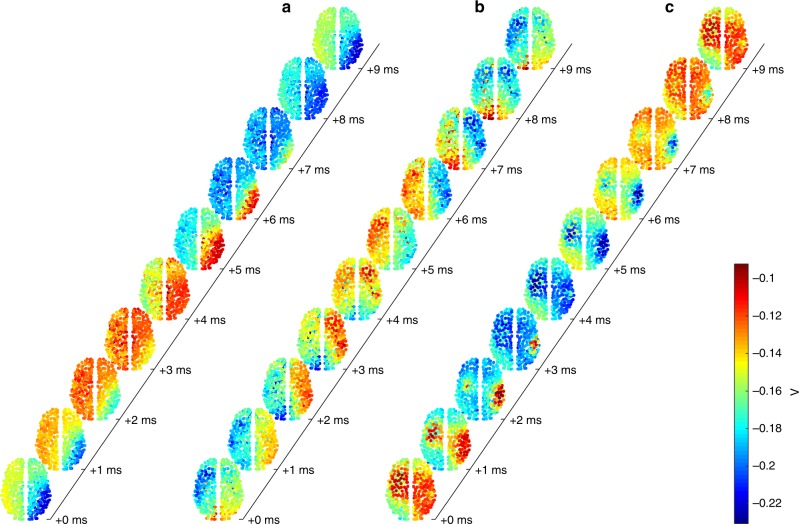
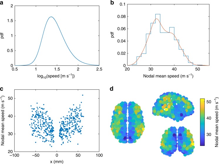
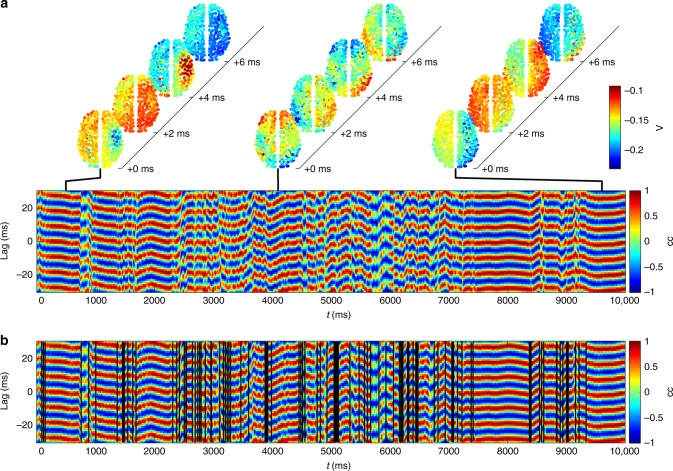
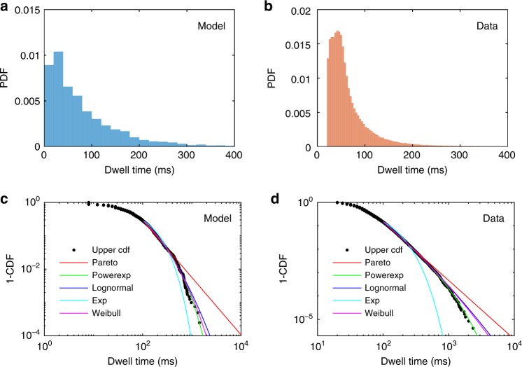
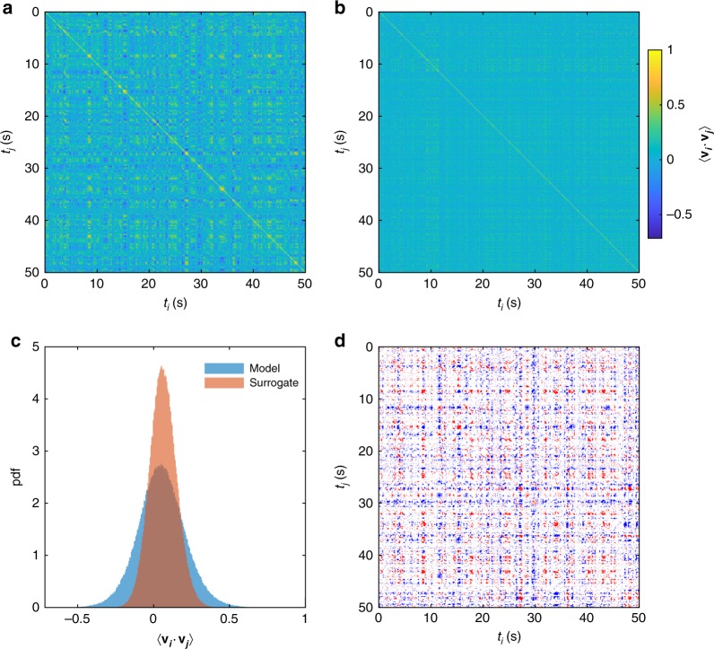
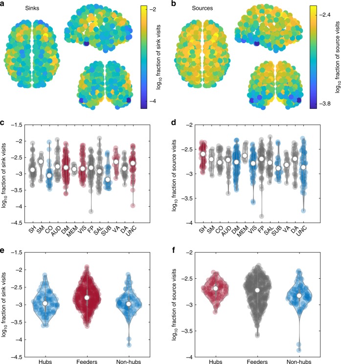
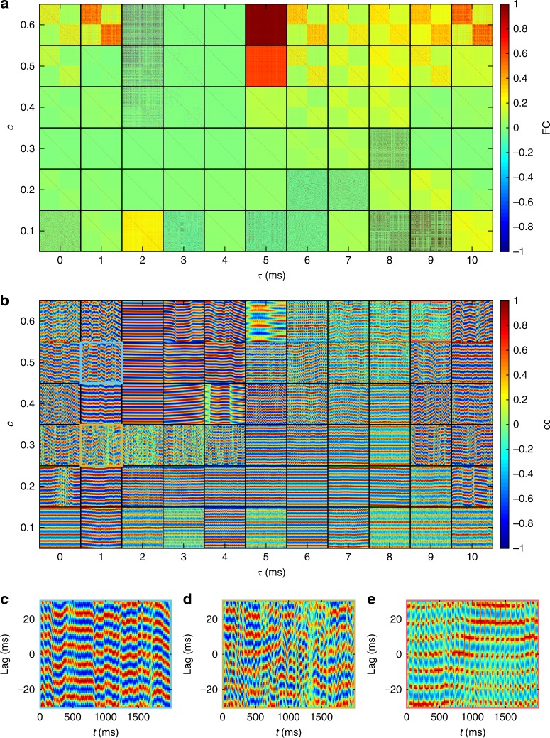
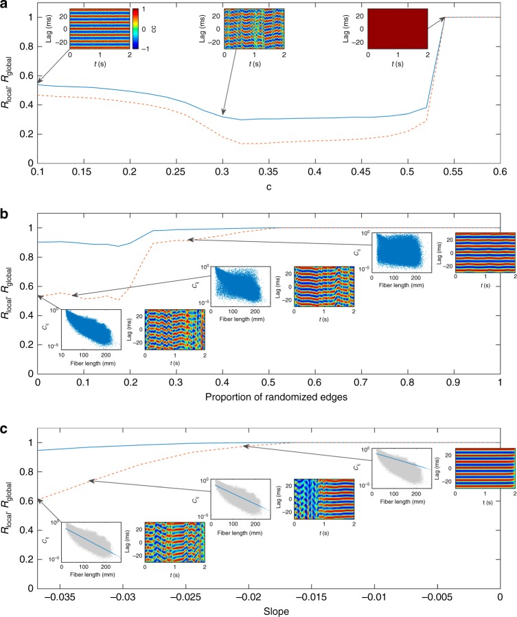
Traveling patterns of neuronal activity-brain waves-have been observed across a breadth of neuronal recordings, states of awareness, and species, but their emergence in the human brain lacks a firm understanding. Here we analyze the complex nonlinear dynamics that emerge from modeling large-scale spontaneous neural activity on a whole-brain network derived from human tractography. We find a rich array of three-dimensional wave patterns, including traveling waves, spiral waves, sources, and sinks. These patterns are metastable, such that multiple spatiotemporal wave patterns are visited in sequence. Transitions between states correspond to reconfigurations of underlying phase flows, characterized by nonlinear instabilities. These metastable dynamics accord with empirical data from multiple imaging modalities, including electrical waves in cortical tissue, sequential spatiotemporal patterns in resting-state MEG data, and large-scale waves in human electrocorticography. By moving the study of functional networks from a spatially static to an inherently dynamic (wave-like) frame, our work unifies apparently diverse phenomena across functional neuroimaging modalities and makes specific predictions for further experimentation.

Fig. 1

Large-scale wave patterns in the model. Ten snapshots of the dynamics of the pyramidal mean membrane potential V at latencies indicated on the time axes, for a a traveling wave, b a rotating wave, and c a pattern with sinks (red areas shrinking for latencies 0–3 ms) and diffuse sources (broad red areas emerging for latencies 6–9 ms). These results are for strong coupling c = 0.6 and short delay τ = 1 ms

Fig. 2

Wave propagation speeds. a Histogram of log₁₀(speed) across all nodes and times. b Histogram of average speed (in m s⁻¹) at each node. Red line shows a kernel density estimate. c Mean speed in each region as a function of the lateral distance from the midline (x = 0). d Spatial distribution of nodal mean speeds as viewed (clockwise from left) from the top, right, and back. These results are for strong coupling c = 0.6 and short delay τ = 1 ms, as in Fig. 1. Source data are provided as a Source Data file

Fig. 3

Metastable transitions. a Each pattern has a signature in the interhemispheric cross-correlation, with transitions between different patterns revealing a brief period of desynchronization. b Vertical lines depict instances of low values of the interhemispheric cross-correlation function, corresponding to wave transitions. These results are for strong coupling c = 0.6 and short delay τ = 1 ms, as in Fig. 1

Fig. 4

Dwell-time distributions. a Model for c = 0.6, d = 1 ms. b Resting-state MEG data from ref. . c, d Upper cumulative distributions (black circles) on double logarithmic axes for dwell times in c the model and d MEG data. Lines are maximum likelihood fits to upper tails for the power law (Pareto, red), exponentially truncated power law (green), lognormal (blue), exponential (cyan), and stretched exponential (Weibull, magenta) distributions. Tail cutoffs at dwell times of 100 ms. Source data are provided as a Source Data file

Fig. 5

Recurring flow patterns. a Recurrences between the mean alignment of velocity fields v_i and v_j at times t_i and t_j, respectively, in the model wave dynamics for c = 0.6, τ = 1 ms. b Recurrences for one instance of an amplitude-adjusted Fourier surrogate time series derived from the simulation used in a. c Histograms of recurrence values for the model (blue) and one surrogate (red). d Recurrence points where the model recurrence alignment was greater than (red) or less than (blue) all 100 surrogates. Red points correspond to flows aligned in the same direction, whereas all blue points correspond to flows aligned in opposite directions

Fig. 6

Phase flow tracked across space and time. a Snapshots of waves (left, colored by voltage as in Fig. 1), the corresponding phase flow vectors (middle, colored by orientation in the 2D plane shown), and phase flow streamlines (right, blue and red denote forward and backward streamlines, respectively). b Exemplar streamlines near metastable transitions, colored as in a, viewed from the top, back, and right (rows 1–3, respectively). Shown are two sets of three snapshots, each surrounding a transition as indicated (gray) in the panel below. Highlighted points (filled circles) denote clusters that form sources (red) and sinks (blue). Black arrows denote the progression of time; colored arrows denote the features referred to in the text. c Lateral positions (displacement from the midline, x) of sinks (top) and sources (bottom) plotted across time, colored by vertical (dorsoventral) position z. Vertical black lines denote transition times calculated using interhemispheric cross-correlation

Fig. 7

Sink and source properties. a Spatial distribution of sinks. b Spatial distribution of sources. c Overlap of sinks with functional networks. Blue denotes networks with fewer visits than red and gray denotes no significant difference from any other group. Networks are labeled as follows: AUD auditory, CO cingulo-opercular, DA dorsal attention, DM default mode, FP fronto-parietal, MEM memory, SAL salience, SH somatomotor hand, SM somatomotor mouth, SUB subcortical, UNC unclassified, VA ventral attention, VIS visual. d Overlap of sources with functional networks. Colors as per c. e Overlap of sinks with hubs (top 75 nodes by strength), feeders, and non-hubs (bottom 75 nodes by strength). Colors as per c. f Overlap of sources with hubs, feeders, and non-hubs. Colors as per c. White circles in violin plots denote group medians; violins are kernel density estimates. Statistics for c, d are given in Supplementary Table 1 and for e, f in Supplementary Table 2. Source data are provided as a Source Data file.

Fig. 8

Dynamics as a function of coupling strength c and delay τ. a Functional connectivity matrices calculated directly from the neuronal time series (corresponding results after convolution of the neuronal time series with a hemodynamic response function are provided in Supplementary Fig. 4). Each tile shows one FC matrix with axes indexing the nodes 1–513. b Interhemispheric cross-correlation functions, showing a 1 s segment (time is on the horizontal axis in each tile) for lags between − 30 ms and 30 ms (lag is on the vertical axis in each tile). Exemplars in the text are highlighted here with colored outlines and shown in corresponding panels: c weakly coherent waves; d interhemispheric cross-correlation dynamics despite negligible average FC; and e lurching waves

Fig. 9

Correlation between modeled and empirical functional connectivity as a function of coupling and delay. a Pearson’s correlation between empirical and modeled FC values for each pair of regions, without GSR. Numbers 1–3 indicate the top three highest correlations. b Same as a but with GSR

Fig. 10

Local and global synchrony for surrogate networks. a Local and global synchrony in fully randomized networks as a function of coupling strength c. Lines show synchronization order parameters R_local (solid) and R_global (dashed). Insets show the interhemispheric cross-correlations at representative values of c, denoted by the arrows. b Loss of waves with progressive structural network randomization, parameterized by the proportion of randomized edges. Insets show the (log-)weight-vs.-fiber length relationships (blue point clouds) and the interhemispheric cross-correlations for the proportion of randomized edges denoted by the arrows. Lines are an average over an ensemble of ten random surrogates at each point. c Waves in synthetic networks with pure exponential weight–distance relationship, parameterized by the slope of the linear log₁₀ (weight)-vs.-fiber length relationship. Insets show the (log-)weight-vs.-fiber length relationships for the synthetic exponential networks (blue) and the original network (gray), and the interhemispheric cross-correlations for the slope values denoted by the arrows. Source data are provided as a Source Data file

References

1. Baker AP, et al. Fast transient networks in spontaneous human brain activity. eLife. 2014;3:e01867. doi: 10.7554/eLife.01867. - DOI - PMC - PubMed
1. Freyer F, Roberts JA, Ritter P, Breakspear M. A canonical model of multistability and scale-invariance in biological systems. PLoS Comput. Biol. 2012;8:e1002634. doi: 10.1371/journal.pcbi.1002634. - DOI - PMC - PubMed
1. Zalesky A, Fornito A, Cocchi L, Gollo LL, Breakspear M. Time-resolved resting-state brain networks. Proc. Natl Acad. Sci. USA. 2014;111:10341–10346. doi: 10.1073/pnas.1400181111. - DOI - PMC - PubMed
1. Muller L, et al. Rotating waves during human sleep spindles organize global patterns of activity that repeat precisely through the night. eLife. 2016;5:e17267. doi: 10.7554/eLife.17267. - DOI - PMC - PubMed
1. Breakspear M, et al. A unifying explanation of primary generalized seizures through nonlinear brain modeling and bifurcation analysis. Cereb. Cortex. 2006;16:1296–1313. doi: 10.1093/cercor/bhj072. - DOI - PubMed
Publication types
LinkOut - more resources