Humans use multi-objective control to regulate lateral foot placement when walking

Abstract

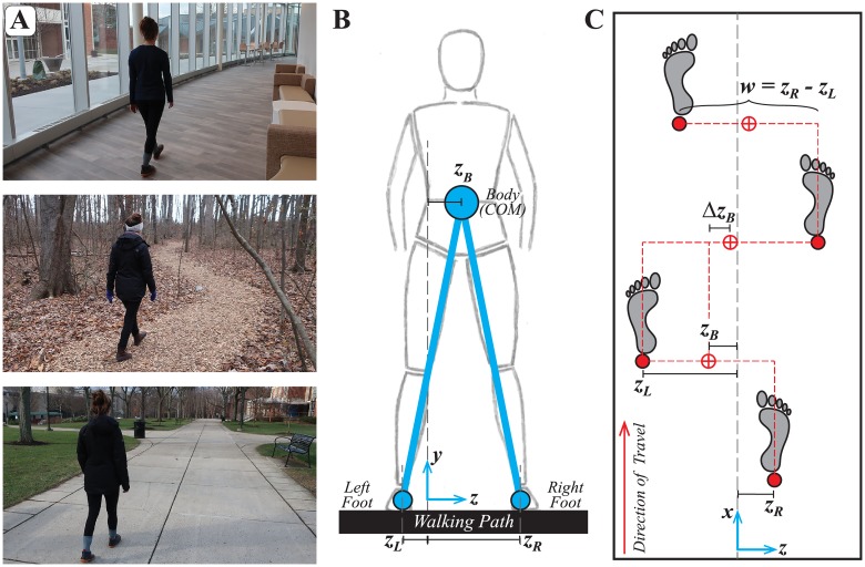
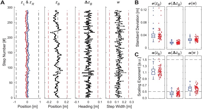
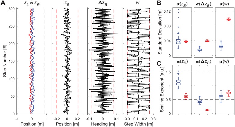
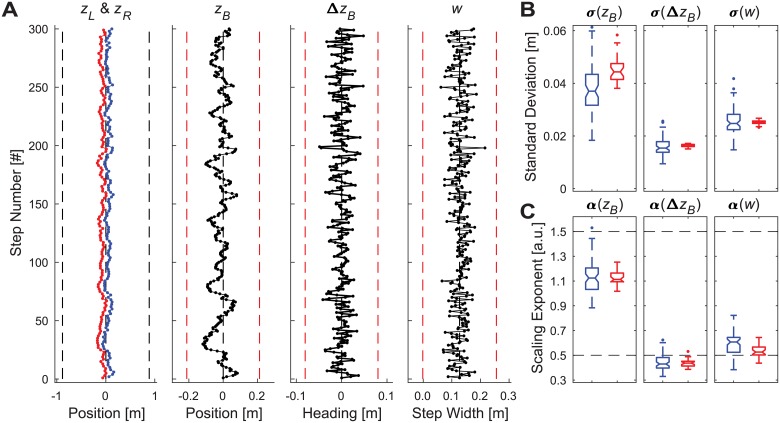
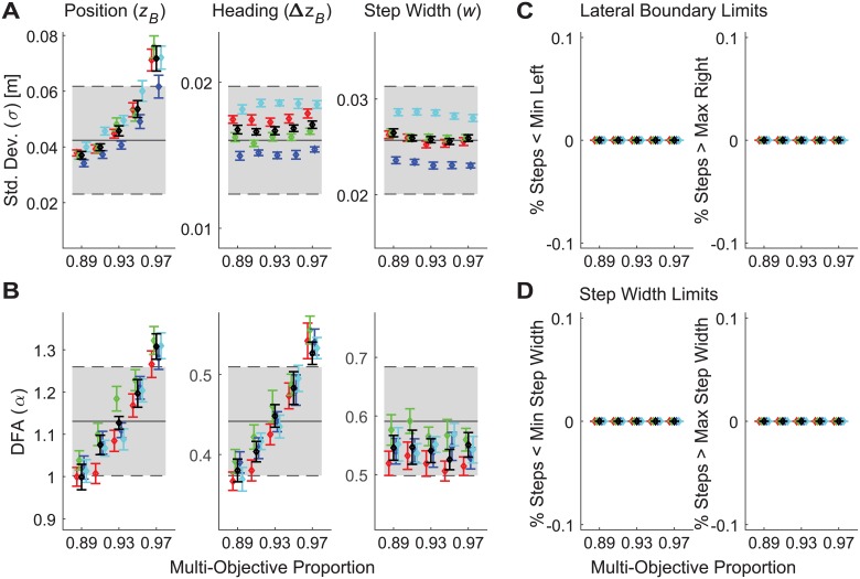
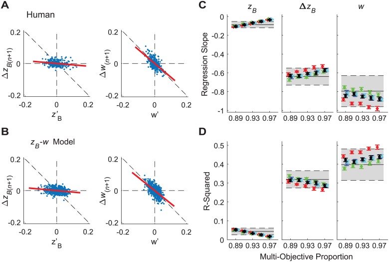
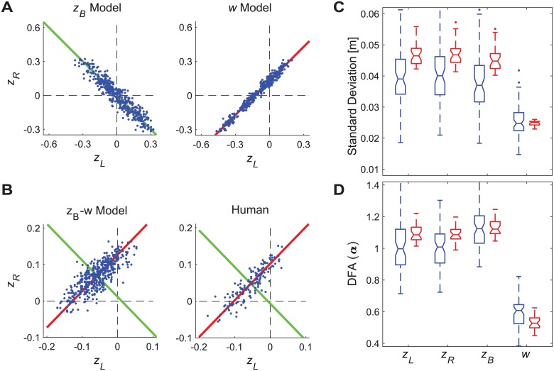
A fundamental question in human motor neuroscience is to determine how the nervous system generates goal-directed movements despite inherent physiological noise and redundancy. Walking exhibits considerable variability and equifinality of task solutions. Existing models of bipedal walking do not yet achieve both continuous dynamic balance control and the equifinality of foot placement humans exhibit. Appropriate computational models are critical to disambiguate the numerous possibilities of how to regulate stepping movements to achieve different walking goals. Here, we extend a theoretical and computational Goal Equivalent Manifold (GEM) framework to generate predictive models, each posing a different experimentally testable hypothesis. These models regulate stepping movements to achieve any of three hypothesized goals, either alone or in combination: maintain lateral position, maintain lateral speed or "heading", and/or maintain step width. We compared model predictions against human experimental data. Uni-objective control models demonstrated clear redundancy between stepping variables, but could not replicate human stepping dynamics. Most multi-objective control models that balanced maintaining two of the three hypothesized goals also failed to replicate human stepping dynamics. However, multi-objective models that strongly prioritized regulating step width over lateral position did successfully replicate all of the relevant step-to-step dynamics observed in humans. Independent analyses confirmed this control was consistent with linear error correction and replicated step-to-step dynamics of individual foot placements. Thus, the regulation of lateral stepping movements is inherently multi-objective and balances task-specific trade-offs between competing task goals. To determine how people walk in their environment requires understanding both walking biomechanics and how the nervous system regulates movements from step-to-step. Analogous to mechanical "templates" of locomotor biomechanics, our models serve as "control templates" for how humans regulate stepping movements from each step to the next. These control templates are symbiotic with well-established mechanical templates, providing complimentary insights into walking regulation.

Fig 1. Defining relevant lateral stepping variables.

A) Common examples of a person walking on paths with lateral boundaries. Such paths occur both indoors and outdoors, can be wide or narrow, may have borders that are more or less well-defined, etc. B-C) Configuration of bipedal walking during a step as viewed in the (B) frontal and (C) horizontal planes. Coordinates are defined in a Cartesian system with {x,y,z} axes as shown in (B) and (C). For convenience, we set the origin at the geometrical center of the path in the lateral direction. Each diagram shows lateral positions of the feet (z_L and z_R) and body (z_B; Eq 2—taken here as a proxy for the center-of-mass, CoM). These yield definitions of primary lateral stepping variables (C) that could be regulated from step to step: positions of the individual feet (z_L and z_R), lateral body position (z_B; Eq 2), change in lateral position (Δz_B; Eq 3), taken here as a proxy for the lateral component of speed or ‘heading’, and step width (w; Eq 4).

Fig 2. Experimental values of primary stepping variables.

A) Example time series data for a representative trial from a typical participant. Each plot shows 290 consecutive steps of left (z_L; red) and right (z_R; blue) foot placements, body position (z_B), heading (Δz_B), and step width (w). For the stepping plot (z_L; z_R), black vertical dashed lines indicate the lateral edges of the treadmill (±0.885 m). For the other time series plots (z_B, Δz_B, and w), red vertical dashed lines indicate ±5 standard deviations, as determined from the average of the standard deviations of all participants. B) Standard deviation (σ) values for all trials for all participants for each variable (z_B, Δz_B, and w). C) DFA scaling exponent (α) values for all trials for all participants for each variable (z_B, Δz_B, and w). For (B) and (C), each subplot shows a summary boxplot (blue–left) indicating the median, 1^st and 3^rd quartiles, and whiskers extending to 1.5× the inter-quartile range, with values beyond that range shown as individual data points. Each subplot also shows individual data points (red dots–right) indicating all individual trials for all participants. These experimental data were aggregated across 65 total trials of 290 steps each, as obtained from 13 participants (5 trials each).

Fig 3. Typical model simulation results for biomechanically constrained position control.

A) Example time series data for a single representative trial. The time series plotted, axes, and axis limits are all the same as in Fig 2. B) Standard deviation (σ) values and (C) DFA scaling exponent (α) values for all trials for each variable (z_B, Δz_B, and w). Each subplot in (B) and (C) shows boxplots (blue–left) and for 30 representative simulated trials from the model (red–right). All boxplots were constructed in the same manner as described in Fig 2. This model failed to replicate experimental findings from humans, as did all other uni-objective control models across all parameter ranges tested (see S1 Appendix for complete details).

Fig 4. Typical model simulation results for multi-objective position-step width control.

A) Example time series data for a single representative trial simulated for baseline parameter values (see S2 Appendix) and a control proportion that was weighted at 93% step width / 7% position control. The time series plotted, axes, and axis limits are all the same as in Fig 2. B) Standard deviation (σ) and (C) DFA scaling exponent (α) values for all trials for each variable (z_B, Δz_B, and w). Each subplot in (B) and (C) shows boxplots for the experimental data (blue–left; from Fig 2) and for 30 representative simulated trials from the model (red–right) using the same parameter values as in (A). All boxplots were constructed in the same manner as described in Fig 2.

Fig 5. Parameter sensitivity results for multi-objective position-step width control.

A) Standard deviations for each primary output variable (z_B, Δz_B, and z_B). B) DFA scaling exponents (α) for each primary output variable. In both (A) and (B), horizontal gray bands indicate the mean ± 1SD band exhibited by humans for that variable to indicate the range of values observed experimentally. For display purposes, all vertical axes are scaled to the mean ± 2SD band exhibited by humans. C) Percentage of steps (z_L and z_R) taken in each simulated trial that exceeded the Lateral Boundary Limits (±0.885 m): i.e., stepped off the treadmill. D) Percentage of steps that exceeded Step Width Limits (±5σ as determined from experimental data; equivalent step width range: −0.15 cm to +25.54 cm), reflecting biomechanically unrealistically wide or narrow steps (see S1 Appendix for details). Stepping data shown here were simulated at multi-objective proportions from 89% step width (11% position) control, every 2% up to 97% step width (3% position) control. Black symbols indicate ‘baseline’ parameter values (see S2 Appendix): σ'_a based on experimental values, σ'_m = 0.1∙σ'_a, and (γ/α)' = 0.1. Red and Green symbols indicate these same baseline parameter values, except γ/α = 0.0 and 0.2, respectively. Blue and Cyan symbols indicate these same baseline parameter values, except σ_a = 0.9∙σ'_a and 1.1∙σ'_a, respectively.

Fig 6. Direct control analysis results for multi-objective position-step width control.

A-B) Example plots of how errors in relative position (z'_Bn) and relative step width (w') were corrected on subsequent strides (Δz_B(n+1) and Δw_(n+1)). Data are shown for (A) one typical experimental trial from typical human participant and for (B) one typical trial from the multi-objective position-step width controller adopting baseline parameter values (see Fig 6). C) Linear regression slopes for each corresponding relationship for each primary output variable (z_B, Δz_B, and z_B). D) Corresponding linear correlation (r²) values for each linear regression for each primary output variable. In both (C) and (D), horizontal gray bands indicate the mean ± 1SD band exhibited by humans for that variable to indicate the range of values observed experimentally. In both (C) and (D), horizontal axis limits and symbol / color designations are the same as shown in Fig 5.

Fig 7. Projection of [z_B, w] control variables onto the [z_L, z_R] stepping plane.

A) Example plots of stepping data for simulations of uni-objective controllers projected onto the [z_L, z_R] plane (see Eq (5)). One typical simulation trial each is shown for controllers regulating either position (z_B) only (left) or step width (w) only (right), each simulated using baseline parameter values (see S1 Appendix). In each plot, diagonal lines indicate the z_B* = constant (green, left) or w* = constant (red, right) GEM’s, as determined from the average position or step width (respectively) exhibited on that trial. All combinations of [z_L, z_R] that lie along either GEM equally satisfy the respective goal. B) Example plots of stepping data for one typical simulated trial from the multi-objective position–step width (z_B-w) controller, simulated using baseline parameter values (see S2 Appendix) and for one typical experimental trial. For each plot, the z_B* and w* GEM’s were determined from the average position and step width exhibited on that trial. C) Standard deviation (σ) and (D) DFA scaling exponent (α) values for all trials for left (z_L) and right (z_R) steps, body position (z_B), and step width (w) for humans (blue) and for the multi-objective position–step width controller, simulated using baseline parameter values (red). All boxplots were constructed in the same manner as described in Fig 2. Note that as all variables are in units of meters, variability measures can be compared directly, as coordinate dependence is not an issue here. All simulation values are well within the range of experimental results. Thus, the multi-objective position–step width control model captured the observed left/right stepping dynamics in [z_L, z_R] as it regulated [z_B, w].

References

1. Stein RB, Gossen ER, Jones KE. Neuronal Variability: Noise or Part of the Signal? Nat Rev Neurosci. 2005;6(5):389–97. 10.1038/nrn1668 - DOI - PubMed
1. Faisal AA, Selen LPJ, Wolpert DM. Noise in the nervous system. Nat Rev Neurosci. 2008;9(4):292–303. 10.1038/nrn2258 - DOI - PMC - PubMed
1. Todorov E, Jordan MI. Optimal feedback control as a theory of motor coordination. Nat Neurosci. 2002;5(11):1226–35. 10.1038/nn963 - DOI - PubMed
1. Scott SH. Optimal Feedback Control and the Neural Basis of Volitional Motor Control. Nat Rev Neurosci. 2004;5(7):532–46. 10.1038/nrn1427 - DOI - PubMed
1. Cohn BA, Szedlák M, Gärtner B, Valero-Cuevas FJ. Feasibility Theory Reconciles and Informs Alternative Approaches to Neuromuscular Control. Front Comput Neurosci. 2018;12:62 10.3389/fncom.2018.00062 - DOI - PMC - PubMed
Publication types