A review of spline function procedures in R

Abstract

Background: With progress on both the theoretical and the computational fronts the use of spline modelling has become an established tool in statistical regression analysis. An important issue in spline modelling is the availability of user friendly, well documented software packages. Following the idea of the STRengthening Analytical Thinking for Observational Studies initiative to provide users with guidance documents on the application of statistical methods in observational research, the aim of this article is to provide an overview of the most widely used spline-based techniques and their implementation in R.

Methods: In this work, we focus on the R Language for Statistical Computing which has become a hugely popular statistics software. We identified a set of packages that include functions for spline modelling within a regression framework. Using simulated and real data we provide an introduction to spline modelling and an overview of the most popular spline functions.

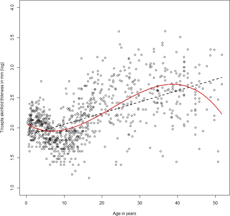
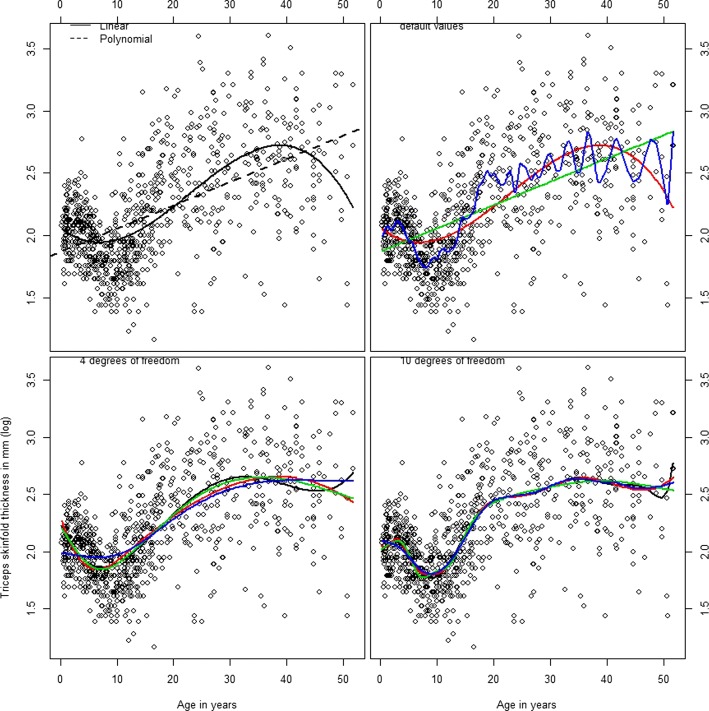
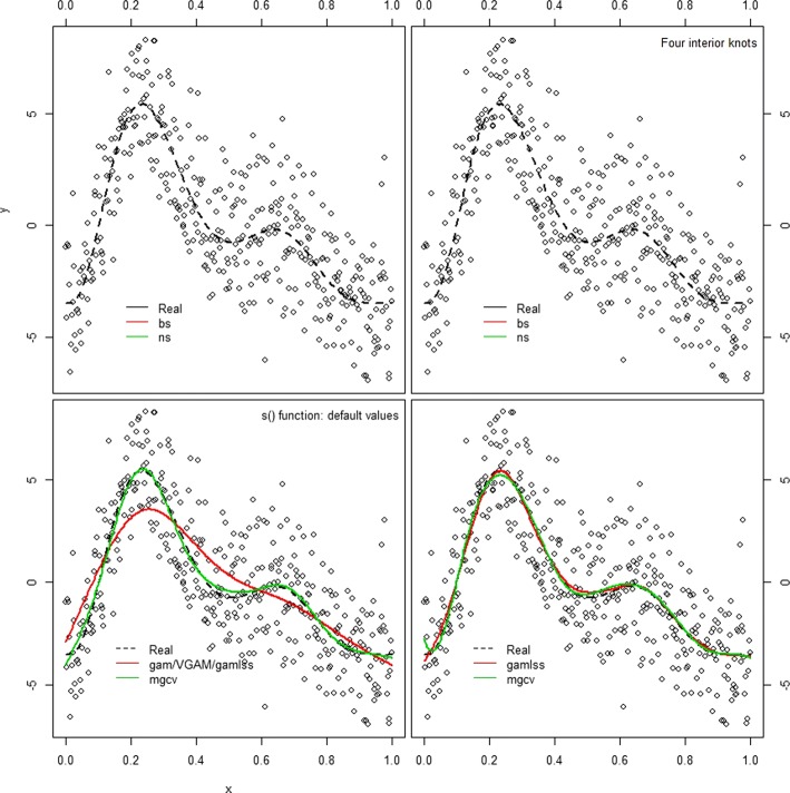
Results: We present a series of simple scenarios of univariate data, where different basis functions are used to identify the correct functional form of an independent variable. Even in simple data, using routines from different packages would lead to different results.

Conclusions: This work illustrate challenges that an analyst faces when working with data. Most differences can be attributed to the choice of hyper-parameters rather than the basis used. In fact an experienced user will know how to obtain a reasonable outcome, regardless of the type of spline used. However, many analysts do not have sufficient knowledge to use these powerful tools adequately and will need more guidance.

Keywords: Functional form of continuous covariates; Multivariable modelling.

Fig. 1

A plot of age in years against the triceps skinfold thickness for 892 females in West Africa [3, 23]. The dashed line represents a simple linear fit, the solid line a fit using flexible third degree polynomials

Fig. 2

Truncated polynomials spline basis functions of third degree (d=3) with five equidistant knots (K=5). Plot created using Code #1 in the Additional file 1: Appendix

Fig. 3

B-spline basis using bs command in library splines. Top left: Spline basis of first degree with three degrees of freedom. Top right: Spline basis of first degree with four degrees of freedom. Bottom left: Cubic spline basis with three degrees of freedom. Bottom right: Cubic spline basis with four degrees of freedom. Graphs created using Code #2

Fig. 4

Natural cubic spline basis using command ns in library splines. Top left: Spline basis with two degrees of freedom. Top right: Spline basis with three degrees of freedom. Bottom left: Spline basis with four degrees of freedom. Bottom right: Spline basis with five degrees of freedom. Created with Code#3

Fig. 5

A plot of age in years against the triceps skinfold thickness for 892 females in West Africa. Upper left: Dashed line represents a simple linear fit, solid line a fit using flexible third degree polynomials. Upper right: Splines fit using default R values. Green line is the result of a polynomial spline of degree 1 (default value for function poly, and a fit from a natural spline with no degrees of freedom specified (default value for functions ns). Red line comes from a b-spline with three degrees of freedom (function bs and blue line from a smoothing spline (from function smooth.spline). Lower left: Black line is polynomial fit, red line b-splines fit, green line is a natural splines fit and smoothing spline, all defined with four degrees of freedom. Lower Right: Same functions defined with 10 degrees of freedom. Created with Code #4

Fig. 6

Scatter plot of simulated data points with different spline fits from packages gam, mgcv and gamlss. Upper left: Data were fitted with library gam that calls B-spline and natural spline functions from splines package. A B-spline with 3 degrees of freedom is the default bs value. Natural splines were used also with three degrees of freedom. The two basis are different, especially in the tails of the x distribution. It is apparent that more flexibility is needed to approach the true curve, given by the dashed line. Upper right: Data fitted with library gam, with added flexibility. Both B-splines and natural splines were defined with four interior knots, resulting in a B-spline with 7 degrees of freedom and a less flexible natural spline with 5 degrees of freedom. Lower left: Comparison of data fitting at default values using function s, in packages mgcv, gam and gamlss. The thin plate regression splines are more flexible than the cubic smoothing spline used by gam and gamlss. Lower right: Comparison of data fitting at default values using P-splines. The differences are rather small and can be attributed to the different way that two packages optimize the penalty weight. Created with Code #6

References

1. Babu GJ. Resampling methods for model fitting and model selection. J Biopharm Stat. 2011;21:1177–86. doi: 10.1080/10543406.2011.607749. - DOI - PubMed
1. Chambers JM, Hastie TJ. Statistical methods in S. Pacific Grove: Wadsworth & Brooks/Cole Advanced Books & Software; 1992.
1. Cole TJ, Green PJ. Smoothing reference centile curves: the lms method and penalized likelihood. Stat Med. 1992;11:1305–19. doi: 10.1002/sim.4780111005. - DOI - PubMed
1. De Boor C. A practical guide to splines. New York: Springer-Verlag; 2001.
1. de Vries A. On the Growth of Cran Packages, r bloggers. 2016. https://www.r-bloggers.com/on-the-growth-of-cran-packages.