COMPOSITIONAL DIVERSITY IN THE ATMOSPHERES OF HOT NEPTUNES, WITH APPLICATION TO GJ 436b

Abstract

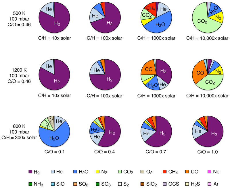
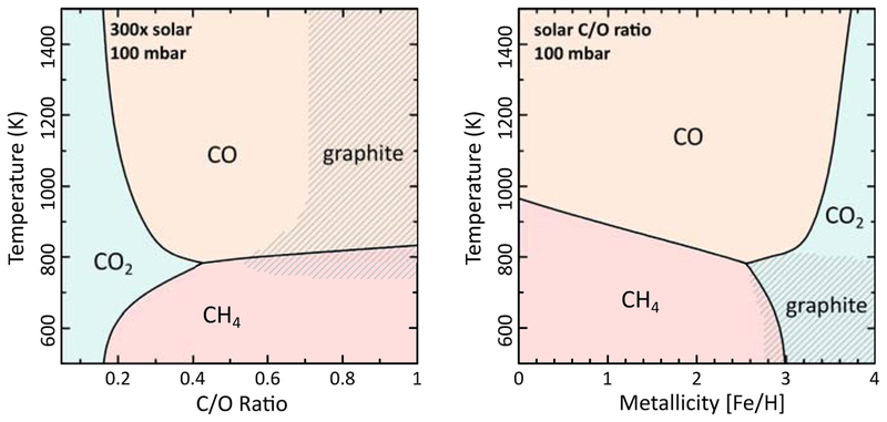
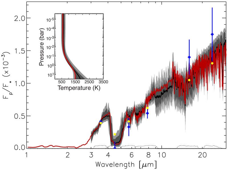
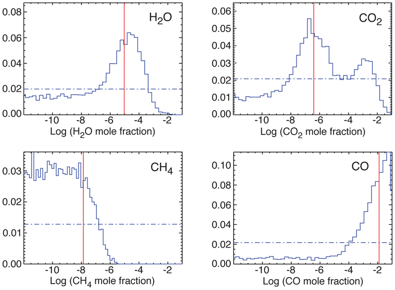
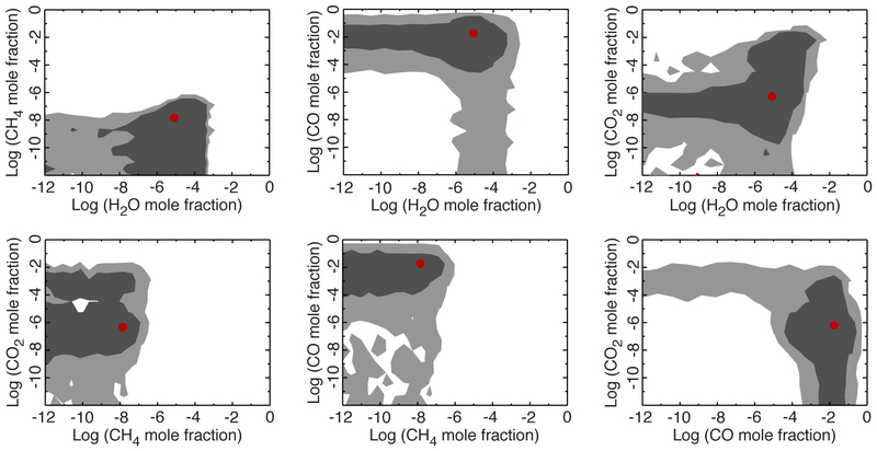
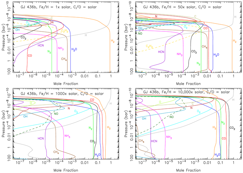
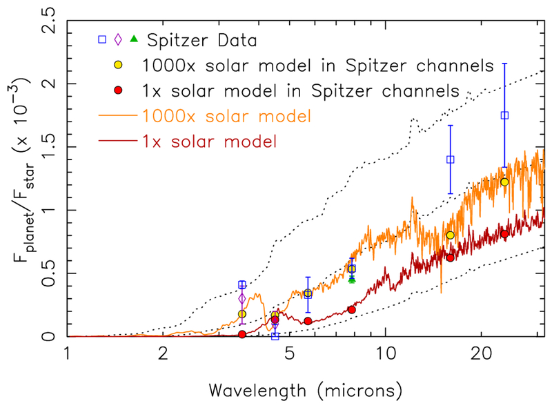
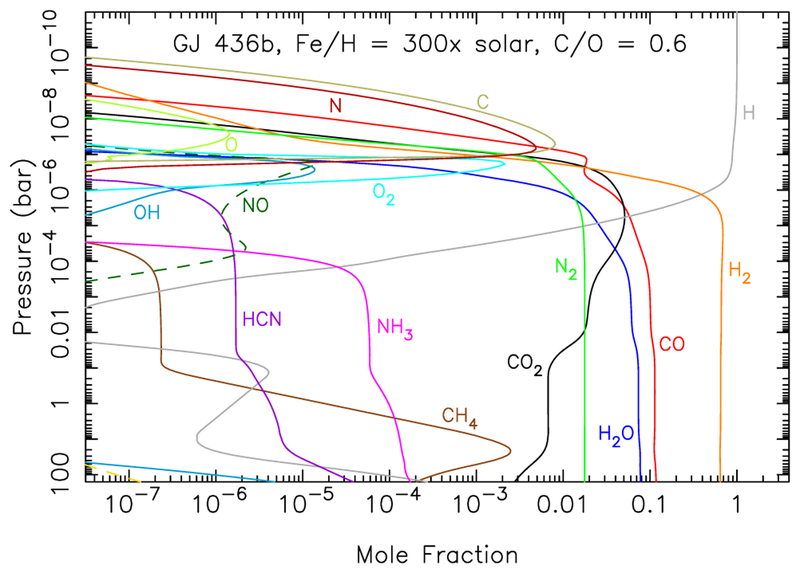
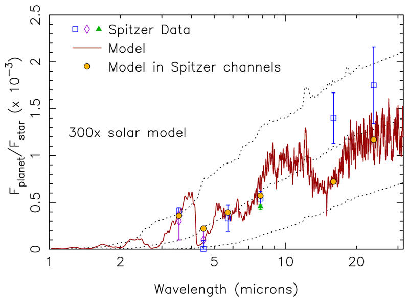
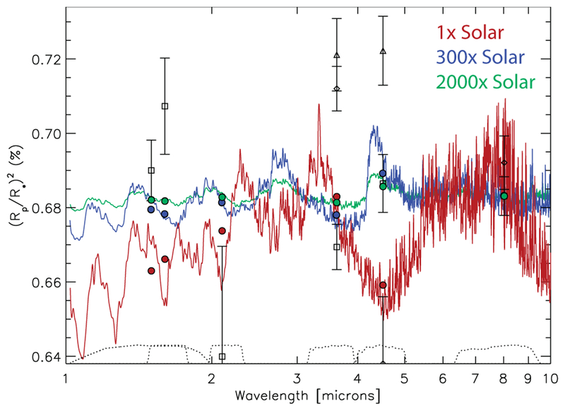
Neptune-sized extrasolar planets that orbit relatively close to their host stars - often called "hot Neptunes" - are common within the known population of exoplanets and planetary candidates. Similar to our own Uranus and Neptune, inefficient accretion of nebular gas is expected produce hot Neptunes whose masses are dominated by elements heavier than hydrogen and helium. At high atmospheric metallicities of 10-10,000× solar, hot Neptunes will exhibit an interesting continuum of atmospheric compositions, ranging from more Neptune-like, H₂-dominated atmospheres to more Venus-like, CO₂-dominated atmospheres. We explore the predicted equilibrium and disequilibrium chemistry of generic hot Neptunes and find that the atmospheric composition varies strongly as a function of temperature and bulk atmospheric properties such as metallicity and the C/O ratio. Relatively exotic H₂O, CO, CO₂, and even O₂-dominated atmospheres are possible for hot Neptunes. We apply our models to the case of GJ 436b, where we find that a CO-rich, CH₄-poor atmosphere can be a natural consequence of a very high atmospheric metallicity. From comparisons of our results with Spitzer eclipse data for GJ 436b, we conclude that although the spectral fit from the high-metallicity forward models is not quite as good as the best fit obtained from pure retrieval methods, the atmospheric composition predicted by these forward models is more physically and chemically plausible in terms of the relative abundance of major constituents. High-metallicity atmospheres (orders of magnitude in excess of solar) should therefore be considered as a possibility for GJ 436b and other hot Neptunes.

Keywords: planetary systems; planets and satellites: atmospheres; planets and satellites: composition; planets and satellites: individual (GJ 436b); stars: individual (GJ 436).

Fig. 1.—

Theoretical thermal profiles (solid lines) for GJ 436b assuming various atmospheric metallicities. The profiles for 1× solar metallicity (blue) and 50× solar metallicity (green) are the atmospheric temperatures averaged over the dayside of GJ 436b at secondary-eclipse conditions from the GCMs of Lewis et al. (2010); the profile for 1000× solar metallicity (red) is from a 1-D, inefficient-heat-redistribution calculation based on Barman et al. (2005). The dashed lines represent the boundaries where CH₄ and CO have equal abundances in chemical equilibrium for the different metallicity models, with the color coding remaining the same as for the thermal profiles. Methane dominates to the lower left of these curves, and CO dominates to the upper right. A color version of this figure is available in the online journal.

Fig. 2.—

Theoretical thermal profiles for GJ 436b assuming different values for the intrinsic internal heat flux $F_{int}=\sigma T_{int}^4$, from 1-D, 50× solar metallicity, inefficient heat redistribution calculations that are based on the models of Fortney et al. (2006, 2007).

Fig. 3.—

Adopted stellar ultraviolet spectrum for GJ 436 (black solid histograms) compared to NGSL spectra of GL 15B (yellow; see Heap & Lindler 2010), IUE spectra of GL 15B (green; Hubble MAST archive), and X-exoplanets theoretical spectra of GJ 436 (cyan; see Sanz-Forcada et al. 2011), all normalized to a distance of 1 AU. A color version of this figure is available in the online journal.

Fig. 4.—

Pie charts illustrating equilibrium gas-phase compositions on generic hot Neptunes for different assumptions about atmospheric properties. The top row shows variations as a function of metallicity (10–10,000 times solar, as labeled) for an atmosphere with a solar C/O ratio, a pressure of 100 mbar, and a temperature of 500 K. The middle row is similar to the top row, except the assumed temperature is 1200 K. The bottom row shows variations as a function of the C/O ratio for an assumed metallicity of 300 times solar (i.e., protosolar abundances of all species except H, He, Ne, and O are multiplied by 300, with O being defined through the C/O ratio), a pressure of 100 mbar, and a temperature of 800 K. Note the very large variation in composition for different bulk atmospheric properties. A color version of this figure is available in the online journal.

Fig. 5.—

Equilibrium mole fractions for different gas-phase species as a function of temperature and metallicity for a solar ratio of elements (except H, He, and Ne remain solar at all metallicities), at a pressure of 100 mbar. When we present a metallicity [X/H] in square brackets here and in subsequent figures, we use the standard logarithmic definition; e.g., a metallicity of [Fe/H] = 3 corresponds to a heavy element enrichment of 1000× solar.

Fig. 6.—

Equilibrium mole fractions for different gas-phase species as a function of temperature and C/O ratio for a 100-mbar pressure and a metallicity X/H = 300× solar (where X represents all elements except H, He, Ne, and O, with the O abundance being defined through the C/O ratio).

Fig. 7.—

Dominant stability regimes in chemical equilibrium at 100 mbar for gas-phase carbon species as a function of temperature and bulk C/O ratio for 300× solar metallicity (left) and as a function of temperature and metallicity for a solar C/O ratio (right). Conditions where graphite is stable are shaded. A color version of this figure is available in the online journal.

Fig. 8.—

Synthetic emission spectra (flux of the planet divided by flux of the star) and thermal profile (insert) for GJ 436b derived from the differential-evolution Markov-chain Monte-Carlo retrieval method described by Line et al. (2013). The span of solutions that fit within 2-sigma (light gray) and 1-sigma (dark gray) are shown in both the temperature-profile and spectral plots, along with the median of the ensemble of fits (black curves). The red curves in both plots represent a single best-fit model. The blue diamonds with error bars are the Spitzer secondary-eclipse photometric data from Stevenson et al. (2010), and the yellow circles show the best-fit model results convolved over the Spitzer bandpasses (with the bandpass sensitivities being plotted as dotted curves near the bottom of the plot). A color version of this figure is available in the online journal.

Fig. 9.—

Gas mole-fraction histograms of the marginalized posterior probability distribution derived from the differential-evolution Markov-chain Monte-Carlo retrieval approach (Line et al. 2013), as applied to the GJ 436b Spitzer eclipse data of Stevenson et al. (2010). The horizontal dot-dashed blue curves represent the priors, which are assumed to be flat (uninformative). The vertical red lines represent the mole fractions that correspond to the best-fit solution. A color version of this figure is available in the online journal.

Fig. 10.—

Contours of the gas-abundance constraints for GJ 436b derived from the differential-evolution MCMC posterior probability distributions, illustrating the correlations between the different gases. The dark gray regions represent the 1-sigma confidence interval and light gray regions represent the 2-sigma confidence interval. The red dot in each plot is the best-fit (maximum-likelihood) solution from the ensemble of 10⁵ fits. A color version of this figure is available in the online journal.

Fig. 11.—

Equilibrium mole fractions for different species as a function of C/H metallicity (see text) and C/O ratio at 900 K and 10 mbar (i.e., a relatively hot, high-altitude photosphere, which may be relevant to a high-metallicity GJ 436b). The shaded region in each plot is where methane has a mole fraction below 10⁻⁶, as is indicated by retrievals based on the Stevenson et al. (2010) Spitzer GJ 436b secondary-eclipse data (our work, and that of Madhusudhan & Seager 2011).

Fig. 12.—

Mixing-ratio profiles for CH₄ (top left), H₂O (top right), CO (bottom left), and CO₂ (bottom right) from our kinetics/transport models for GJ 436b, for assumed atmospheric metallicities of 1× solar (blue solid lines), 50× solar (green solid lines), 1000× solar (orange solid lines), and 10,000× solar (purple solid lines), as described more fully in Fig. 13. The corresponding equilibrium solutions for the 10,000× solar model are shown as dashed purple lines. The red horizontal bar illustrates the most-probable solutions derived from the differential-evolution MCMC approach discussed in section 3.2, with the star representing the best-fit solution. The black horizontal bar represents the model solutions from Madhusudhan & Seager (2011) that fit the Spitzer data to within χ²/N_obs ≤ 1. Note that none of the disequilibrium models for the different metallicities have mole fractions that fall within the retrieval constraints for all four species. A color version of this figure is presented in the online journal.

Fig. 13.—

Mixing-ratio profiles for several species of interest (as labeled) in our kinetics/transport models for GJ 436b, for assumed atmospheric metallicities of 1× solar (top left), 50× solar (top right), 1000× solar (bottom left), and 10,000 solar× (bottom The thermal profiles adopted in these models are described in section 2.2 right). (see Fig. 1); the profile for the 10,000× solar model (not shown in Fig. 1) was derived from the PHOENIX model (Hauschildt et al. 1999; Allard et al. 2001; Barman et al. 2005) and is very similar to the 1000× solar profile. The C/O ratio is assumed to be the protosolar value of Lodders et al. (2009) with 21% of the oxygen unavailable due to being bound up in condensates at deep atmospheric levels (Visscher et al. 2010a), and the eddy diffusion coefficient K_zz is assumed to be constant at 10⁹ cm² s⁻¹. A color version of this figure is presented in the online journal.

Fig. 14.—

Synthetic emission spectra for GJ 436b for our disequilibrium models that assume a 1× solar metallicity atmosphere (dark red) and a 1000× solar metallicity atmosphere (orange), in comparison with observations (data points with error bars). The thermal profiles assumed in the models are shown in Fig. 1, and the abundance profiles are shown in Fig. 13. The blue squares represent the Spitzer secondary-eclipse data analyzed by Stevenson et al. (2010), with an updated upper limit at 4.5-μm from Stevenson et al. (2012), the purple diamonds represent the Beaulieu et al. (2011) analysis of the same 3.6 and 4.5-μm data, and the green triangle represents the analysis of 11 secondary eclipses of GJ 436b in the 8-μm channel by Knutson et al. (2011). The red and gold circles represent, respectively, the fluxes from the 1× and 1000× solar models, averaged over the Spitzer bandpasses. The black dotted lines represent the planetary emission (smoothed) assuming GJ 436b radiates as a blackbody at a temperature of 500 K (lower curve), 800 K (middle curve), or 1100 K (upper curve). The apparent emission “spikes” represent stellar absorption, as everything here is plotted in terms of the flux of the planet divided by the flux of the star. A PHOENIX stellar model (e.g., Hauschildt et al. 1999) with T_eff = 3350 K was assumed for the host star for all these calculations. A color version of this figure is available in the online journal.

Fig. 15.—

Mixing-ratio profiles for several species of interest (as labeled) in our kinetics/transport models for GJ 436b, for an assumed atmospheric metallicity of 300× solar in carbon and nitrogen, with the oxygen elemental abundance defined through an assumed C/O ratio of 0.6. The eddy diffusion coefficients are taken to be K_zz = 10⁷ cm² s⁻¹ at P ≥ 10⁻⁴ bar, with K_zz increasing as the inverse square root of the pressure at P < 10⁻⁴ bar. The thermal profile is taken from Fig. 4 of Madhusudhan & Seager (2011), but we have shifted the entire profile upwards uniformly in an attempt to account for the higher-altitude photosphere with higher metallicities (see text). A color version of this figure is available in the online journal.

Fig. 16.—

Synthetic emission spectra (dark red) for GJ 436b for our disequilibrium model that assumes a 300× solar metallicity atmosphere, with a C/O ratio of 0.6 (see text and Fig. 15). The blue squares represent the Spitzer secondary-eclipse data analyzed by Stevenson et al. (2010), with an updated upper limit at 4.5-μm from Stevenson et al. (2012), the purple diamonds represent the the 3.6 and 4.5-μm Spitzer analysis of Beaulieu et al. (2011), and the green triangle represents additional Spitzer eclipse data at 8-μm as analyzed by Knutson et al. (2011). The red circles represent the model fluxes averaged over the Spitzer bandpasses. The black dotted lines represent the planetary emission assuming GJ 436b radiates as a blackbody at a temperature of 500 K (lower curve), 800 K (middle curve), or 1100 K (upper curve). See Fig. 14 for further details. A color version of this figure is available in the online journal.

Fig. 17.—

Synthetic transmission spectra for GJ 436b (in terms of the apparent transit depth, i.e., the square of the ratio of the planetary radius to the stellar radius) for our disequilibrium models that assume a 1× (red), 300× (blue), and 2000× (green) solar metallicity. Scattering from molecules or hazes is not included in the calculations. Data points from various sources are shown in black, with associated error bars. In order of increasing wavelength, the squares are from the 1.1–1.9 μm HST/NICMOS analysis of Pont et al. (2009) plotted at 1.5 μm; the ground-based H-band data of Alonso et al. (2008) plotted at 1.6 μm; the ground-based K_s band data of Cáceres et al. (2009) plotted at at 2.1 μm, as discussed by Knutson et al. (2011); and the Spitzer/IRAC analysis of Knutson et al. (2011) plotted at 3.6, 4.5, and 8 μm. The diamonds are from the Spitzer analysis of Beaulieu et al. (2011) at 3.6, 4.5, and 8 μm. The triangles are the Spitzer transits at 3.6 and 4.5 μm that Knutson et al. (2011) suggest are influenced by the occultation of star spots or other regions of non-uniform brightness on the star. The black dotted curves at the bottom show the response functions for the filters and/or detector channels used in the observations. The colored circles represent the corresponding model transit depths averaged over the appropriate filters/channels. A color version of this figure is available in the online journal.

Fig. 18.—

Constraints on the bulk composition of GJ 436b as determined from models of its structure, evolution, and formation. Possible compositions are shown for six different model assumptions and/or imposed constraints. For each, the sum over the displayed mass fractions of H/He (green diamonds), water (blue squares), and “rock” (includes silicates plus iron; orange triangles) equals 1. All calculations take into account the planet’s mass M_p and radius R_p as one set of constraints; the two leftmost models consider uncertainties in M_p and R_p, which expands the possible H/He mass fraction by a factor of ~2, while the four on the right adopt specific M_p and R_p values from Torres et al. (2008). From left to right, the derived constraints are based on (i) the thermal and structural evolution models of Miller & Fortney (2011) that assume an ice:rock ratio of 1:1 and that impose constraints based on the age of the GJ 436 system; (ii) the formation, disk-planet evolution (including migration), and structural models of Figueira et al. (2009) that compute various formation paths consistent with M_p and R_p; (iii) the structure models of Adams et al. (2008) that consider precise values for M_p, R_p, and atmospheric temperatures and thus derive a smaller range of acceptable H/He values; (iv) the structural models of Nettelmann et al. (2010) that assume that water is mixed into the outermost H/He envelope; (v) structural models based on Nettelmann et al. (2010) that assume that a pure H/He layer resides above a water layer with a warm (1300 K) deep isothermal radiative region; (vi) a model similar to the one on the immediate left, except the isothermal radiative region is cool (700 K) and the planet is old (> 10 Gyr). Note from comparing the latter two models that atmospheric temperatures affect the derived H/He mass fraction. A color version of this figure is available in the online journal.

References

1. Adams ER, Seager S, & Elkins-Tanton L 2008, ApJ, 673, 1160
1. Agúndez M, Venot O, Iro N, et al. 2012, A&A, 548, A73
1. Alibert Y, Mordasini C, Benz W, & Winisdoerffer C 2005, A&A, 434, 343
1. Alibert Y, Baraffe I, Benz W, et al. 2006, A&A, 455, L25
1. Allard F, Hauschildt PH, Alexander DR, Tamanai A, & Schweitzer A 2001, ApJ, 556, 357