Resting-state brain information flow predicts cognitive flexibility in humans

Abstract

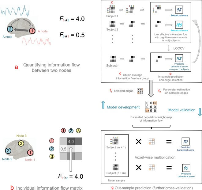
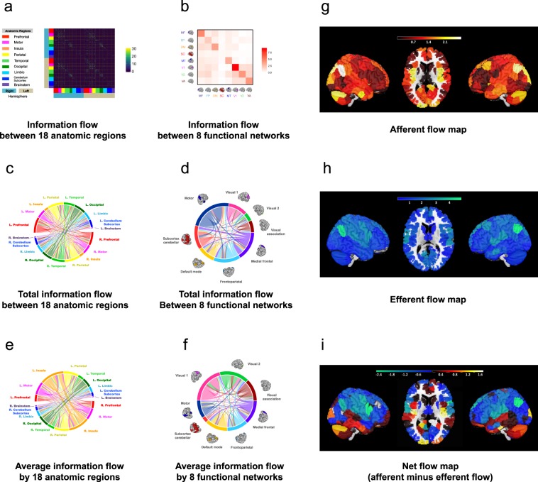
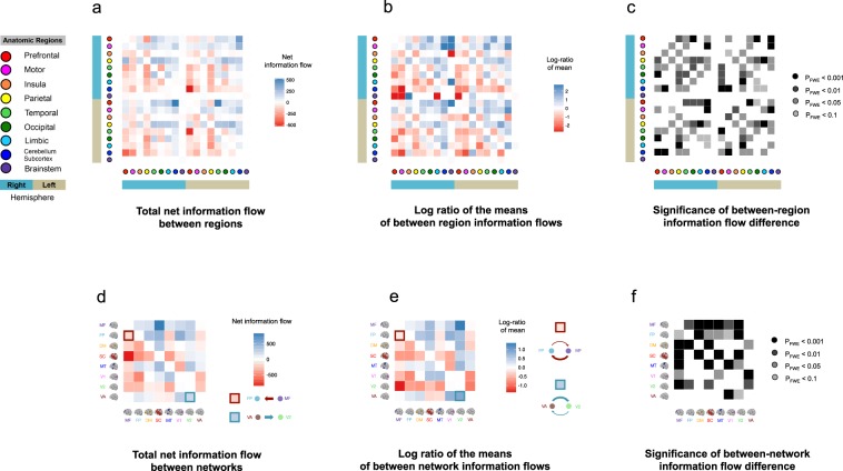
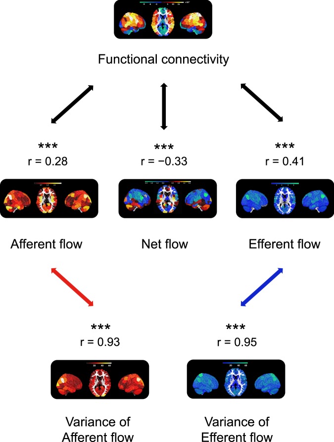
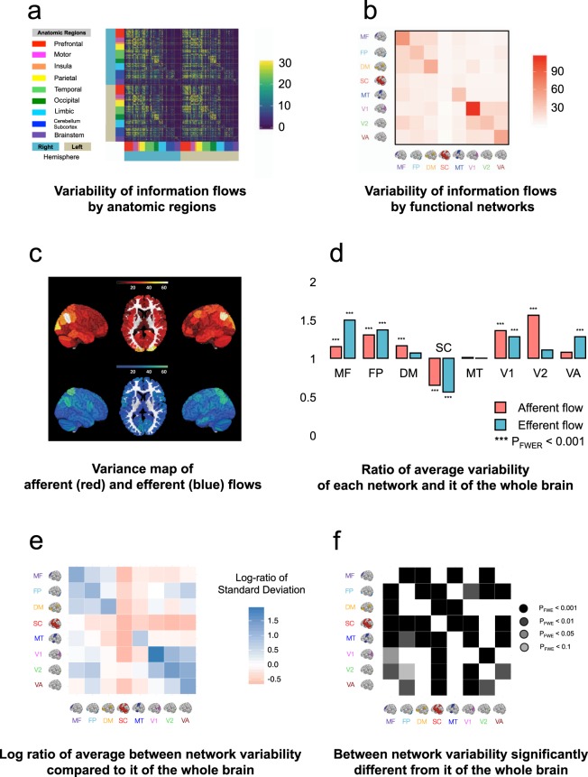
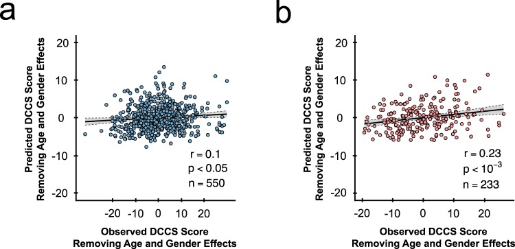
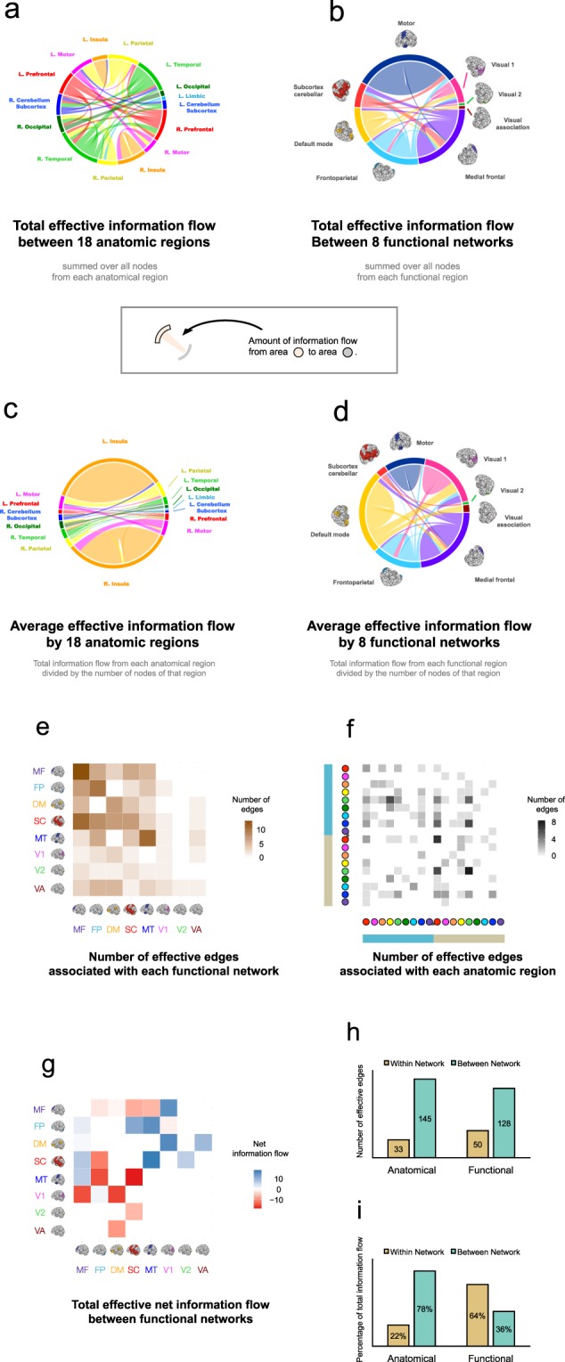
The human brain is a dynamic system, where communication between spatially distinct areas facilitates complex cognitive functions and behaviors. How information transfers between brain regions and how it gives rise to human cognition, however, are unclear. In this article, using resting-state functional magnetic resonance imaging (fMRI) data from 783 healthy adults in the Human Connectome Project (HCP) dataset, we map the brain's directed information flow architecture through a Granger-Geweke causality prism. We demonstrate that the information flow profiles in the general population primarily involve local exchanges within specialized functional systems, long-distance exchanges from the dorsal brain to the ventral brain, and top-down exchanges from the higher-order systems to the primary systems. Using an information flow map discovered from 550 subjects, the individual directed information flow profiles can significantly predict cognitive flexibility scores in 233 novel individuals. Our results provide evidence for directed information network architecture in the cerebral cortex, and suggest that features of the information flow configuration during rest underpin cognitive ability in humans.

Figure 1

A flow chart for extracting population information map and conducting out-of-sample prediction for cognitive measurement using information flow in the human brain. (a) Obtaining information flow metrics (F-values) between every pair of regions. For time courses from brain regions 1 and 2, we obtained two directed values F_1→2 (information flow from region 1 to 2) and F_2→1 (information flow from region 2 to 1). (b) Arranging F-values as an information flow matrix. Specifically, F-values obtained from (a) were arranged corresponding to brain regions in an asymmetrical matrix. (c) Obtaining individual information flow matrix. For every subject, we computed the F-values for every pair of time courses. This yielded a 268 × 268 subject-specific asymmetrical F-value matrix and a 268 × 268 asymmetrical p-value matrix (corresponding to the F-value matrix) for each subject. (d) Obtaining average information flow in a group. We first computed the average p-values for edge across subject. We recorded edges with corresponding F-values that had an average p-value less than a threshold (e.g. 0.05). (e) Edge (F-value) selection. We used a two-step feature selection procedure. During the first step, we selected an F-value if its average p-values across subjects were below a threshold (see Methods for details). We then used a leave-one-subject-out cross-validation (LOOCV) analysis to conduct a further feature selection on F-values, and build a predictive model. The training and testing in LOOCV were performed iteratively for n times. (f₁) Due to the large variability of LOOCV, we took the union of the selected features from each LOOCV iteration. (f₂) Using selected F-values, we built a feature weight map of information flow. (g) Out-of-sample prediction. We multiplied the information weight map with F-values from previously unseen subjects, without further model fitting, to predict their cognitive scores. The efficacy and predictive power of information flow in predicting cognitive flexibility was evaluated by correlating the predicted and observed cognitive measurements.

Figure 2

Average whole-brain information flow in a group. (a) The 268 × 268 asymmetrical information flow matrix averaged from 550 individual information matrices. The matrix is defined on 18 anatomic regions using a 268-node functional atlas. The atlas is based upon an independent data set of healthy control subjects using a group-wise spectral clustering algorithm. Every entry contains a selected F-value from the lag-adjusted Granger-Geweke test between two time courses, or 0, if the F-value is not selected. An edge is selected if its average p-value across all subjects is smaller than 0.05. (b) The 8 × 8 asymmetrical information flow matrix defined on 8 functional networks. The value for each entry is the mean F-values associated with a functional brain network summarized from the 268 × 268 matrix in (a). (c) Total information flow map between 18 anatomic regions. The map contains 3,927 significant directed edges organized on 18 regions as in (a). The color of the edge indicates the origin of the flow. For example, the red curved line crossing the circle starting from the left (red bar) to the lower right (light orange bar) indicates information flow from left prefrontal region to right insula region. (d) Total information flow map between 8 functional networks. The same 3,927 edges in (c) now visualized on 8 functional brain networks. (e) Average information flow between 18 anatomic regions. The total amount of information flow from each anatomic region specified in (c) divided by the number of node in the region. (e) Average information flow between 8 functional networks. The total amount of information flow from each functional network specified in (d) divided by the number of node in the region. (g–i) Afferent, efferent, and net information flow maps of the whole brain. The brain images in (b, d and f) are adapted by permission from RightsLink Permissions Springer Customer Service Centre GmbH: Springer Nature Neuroscience “Functional connectome fingerprinting: identifying individuals using patterns of brain connectivity” by Finn et al. Copyright 2015.

Figure 3

Net total information flows of the whole-brain and mean information flow difference between regions and networks. (a) The net total information flows of the whole brain organized by regions. Each square represents the net total amount of information flows from one brain area to the other. The darker a blue square was, then the more (net) information was flowing out from the brain region denoted by the reference brain image on the horizontal direction into the brain area denoted by the reference brain image on the vertical direction. The darker a red square was, the more (net) information was flowing into the brain region denoted by the reference brain image on the horizontal direction from the region denoted by the reference brain image on the vertical direction. (b) The mean difference between region information flows. Each square represents the difference between the mean of information flows from the brain area denoted by the reference brain image on the horizontal direction to the brain area denoted by the reference brain image on the vertical direction. Color conventions as in (a). (c) The p-values for the corresponding mean difference in (b), corrected by FWER. (d) The net total information flows of the whole brain organized by networks. Color conventions as in (a). (e) The mean difference between network information flows. Color conventions as in (a). (f) The p-values for the corresponding mean difference in (e), corrected by FWER. The brain images in (d, e and f) are adapted by permission from RightsLink Permissions Springer Customer Service Centre GmbH: Springer Nature Neuroscience “Functional connectome fingerprinting: identifying individuals using patterns of brain connectivity” by Finn et al. Copyright 2015.

Figure 4

A comparison between functional and effective connectivity. The functional connectivity map was obtained by first averaging 550 268 × 268 Pearson correlation matrices obtained from 550 subjects. Subsequently, the resulting 268 × 268 matrix was further summarized according to 268 brain areas. This yielded a vector containing 268 values, each of which corresponds to the “connectiveness” of a brain area to the rest of brain areas. The effective connectivity map was obtained by first averaging 550 268 × 268 F-matrices obtained from 550 subjects. Subsequently, the resulting 268 × 268 matrix was further summarized according to 268 brain areas, into three vectors. The first vector contained 268 values, each of which corresponds to how much information flow is flowing into a particular brain area from other brain areas (afferent flow). The second vector also contained 268 values, each of which corresponds to how much information flow was flowing out from a particular brain area to other brain areas (efferent flow). The third vector was obtained by subtracting the efferent flow from the afferent flow, indicating the net information flow entering each brain area. Finally, the association between functional and effective connectivities can be quantified by correlating the functional connectivity vector with each of the three effective connectivity vectors.

Figure 5

Analysis of variance of the whole-brain information flows. (a) The variance of 268 × 268 asymmetrical information flow map across 550 subjects. Every entry contains the variance of the F-value between two time courses across subjects. In the figure, for color contrast convenience, if an F-value is greater than 100, we fix it at 100. (b) The variance of 8 × 8 asymmetrical information flow map across all subjects defined on 8 functional networks. Every entry is the mean variance of F-value associated with a functional brain network summarized from the 268 × 268 matrix in (a). (c) The variability map of afferent (in red color) and efferent flows (in blue color). (d) The variability of afferent (red) and efferent flows (blue) associated with each network compared to it of the whole brain. The height of each histogram quantifies the average variance of F-values corresponds to each network, which were visualized in panel (c), compared to it of the whole brain. A pair-wise ANOVA test determines the significance level. All p-values were adjusted for FWER. (e) The log-ratio of average variation of information flows between each pair of networks. Each log-ratio was calculated in two steps. First, we found the average variations of the efferent flow from nodes linking regions A and B - it measures the average variability of the efferent flow from region A to region B. We also found the average variations of the afferent flow from regions B to A - it measures the average variability of the afferent flow from region A to region B. Second, we calculated the natural log of these two average variations. The darker a blue square was, the more variability of information flowing out from the brain region denoted by the reference brain image on the horizontal direction than the variability of the opposite information flows; the darker a red square was, the more variability of information flowing into the brain region denoted by the reference brain image on the horizontal direction than the variability of the opposite information flows. (f) The significance of the between-network variability. The darker the green square, there was more significant a difference between the variability of the information flows from opposite directions (namely, the variability of information flow from region A to B compared to it from region B to A). The size of the difference (namely, whether there is more variability of the information flow from region A to B than it from B to A) can be determined from the map in (e). The comparison was done using a pair-wise ANOVA test. All p-values were adjusted for FWER. The brain images in (e) and (f) are adapted by permission from RightsLink Permissions Springer Customer Service Centre GmbH: Springer Nature Neuroscience “Functional connectome fingerprinting: identifying individuals using patterns of brain connectivity” by Finn et al..

Figure 6

Individual effective information flow predicts cognitive flexibility. (a) LOOCV prediction result comparing predicted and observed DCCS scores (n = 550 subjects). Confounds, such as age and gender, are regressed out before prediction. Scatter plot shows predication based upon the whole brain positive effective information flows (threshold at p < 0.005). Each dot represents one subject; grey area indicates the 95% confidence band for best-fit line. (b) Out-of-sample prediction result comparing predicted and observed adjusted DCCS scores (n = 233 subjects). Confounds, such as age and gender, are regressed out before prediction. Scatter plot shows predication based upon the whole brain positive effective information flows (threshold at p < 0.005). Each dot represents one subject; grey area indicates the 95% confidence band for best-fit line.

Figure 7

Individual effective information flows. (a) The information map of positive total effective information flow edges based upon feature selection. The flows are arranged according to 18 brain regions. (b) The same edges in (a) now organized according to 8 functional brain networks. (c) Average effective information flow (total effective information flow in figure (a) divided by the number of nodes in each anatomic region). (d) Average effective information flow (total effective information flow in figure (b) divided by the number of nodes in each functional network). (e) Number of effective edges arranged according to 8 functional brain regions. (f) Number of effective edges arranged according to 18 anatomic brain regions. Color convention as in Fig. 3 (a). (g) Net total effective information flow between 8 functional brain regions. The darker the black square was, then the more information is flowing out from the brain region denoted by the reference brain image on the horizontal direction to the brain region denoted by the reference brain image on the vertical direction; the darker the red was, then the more information is flowing into the brain region denoted by the reference brain image on the horizontal direction from the brain region denoted by the reference brain image on the vertical direction. (h) The number of effective edges arranged by within and between anatomic regions, as well as it arranged by within and between functional networks. (i) The total information flow (summed F-values) arranged by within and between anatomic regions, as well as it arranged by within and between functional networks. The brain images are adapted by permission from RightsLink Permissions Springer Customer Service Centre GmbH: Springer Nature Neuroscience “Functional connectome fingerprinting: identifying individuals using patterns of brain connectivity” by Finn et al..

References

1. Finn ES, et al. Functional connectome fingerprinting: identifying individuals using patterns of brain connectivity. Nat Neurosci. 2015;18:1664–1671. doi: 10.1038/nn.4135. - DOI - PMC - PubMed
1. Rosenberg, M. D. et al. A neuromarker of sustained attention from whole-brain functional connectivity. Nat Neurosci19, 165–171, 10.1038/nn.4179, http://www.nature.com/neuro/journal/v19/n1/abs/nn.4179.html - supplementary-information (2016). - PMC - PubMed
1. Friston KJ. Functional and effective connectivity in neuroimaging: a synthesis. Human brain mapping. 1994;2:56–78. doi: 10.1002/hbm.460020107. - DOI
1. Friston KJ. Functional and effective connectivity: a review. Brain connectivity. 2011;1:13–36. doi: 10.1089/brain.2011.0008. - DOI - PubMed
1. Hillebrand A, et al. Direction of information flow in large-scale resting-state networks is frequency-dependent. Proceedings of the National Academy of Sciences. 2016;113:3867–3872. doi: 10.1073/pnas.1515657113. - DOI - PMC - PubMed
Publication types