Higher-Order Thalamic Circuits Channel Parallel Streams of Visual Information in Mice

Abstract

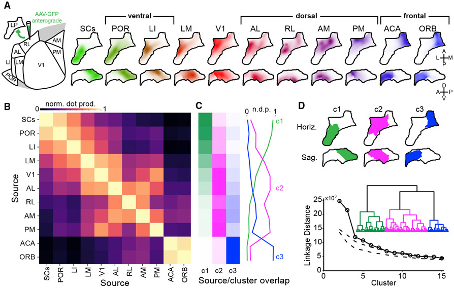
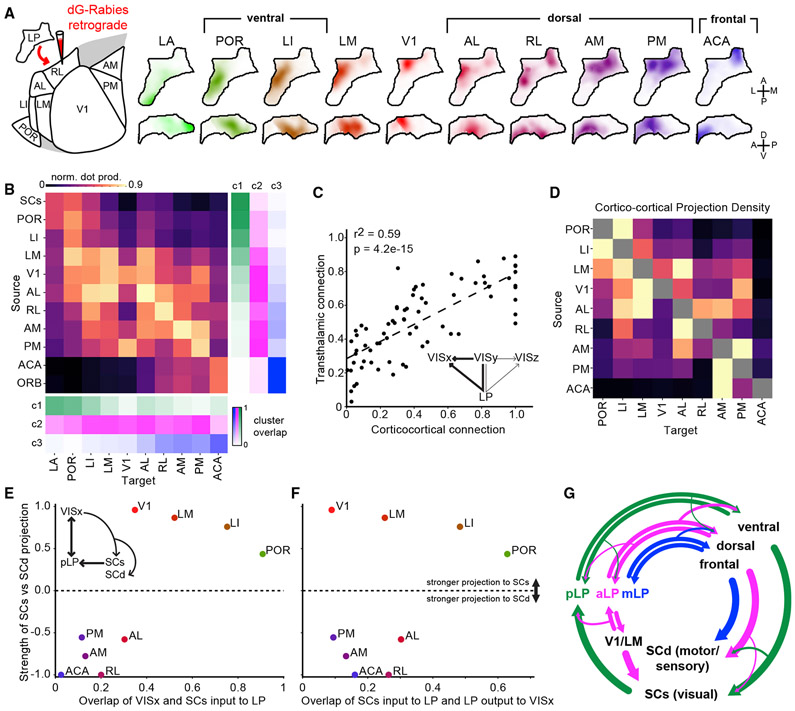
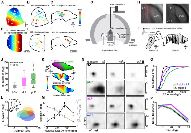
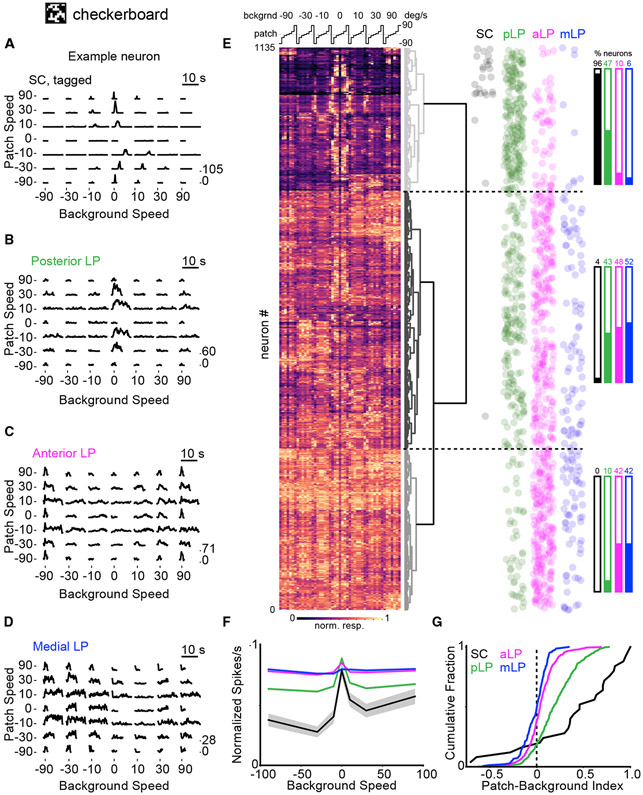
Higher-order thalamic nuclei, such as the visual pulvinar, play essential roles in cortical function by connecting functionally related cortical and subcortical brain regions. A coherent framework describing pulvinar function remains elusive because of its anatomical complexity and involvement in diverse cognitive processes. We combined large-scale anatomical circuit mapping with high-density electrophysiological recordings to dissect a homolog of the pulvinar in mice, the lateral posterior thalamic nucleus (LP). We define three broad LP subregions based on correspondence between connectivity and functional properties. These subregions form corticothalamic loops biased toward ventral or dorsal stream cortical areas and contain separate representations of visual space. Silencing the visual cortex or superior colliculus revealed that they drive visual tuning properties in separate LP subregions. Thus, by specifying the driving input sources, functional properties, and downstream targets of LP circuits, our data provide a roadmap for understanding the mechanisms of higher-order thalamic function in vision.

Keywords: lateral posterior thalamic nucleus; pulvinar; superior colliculus; thalamus; visual cortex.

Figure 1.. Input Connectivity Reveals Three Broad LP Subregions

(A) Left: schematic of input mapping experiments, showing visual cortical areas in the horizontal plane. Right: location of anterogradely labeled axons in LP from various cortical and subcortical input sources. Input volumes are shown as horizontal (top row) and sagittal projections (bottom row) and represent average fluorescence across multiple tracer injection experiments registered in the Allen Mouse Common Coordinate Framework (STAR Methods). (B) Overlap of inputs to LP from different sources (normalized voxel-wise dot product). (C) Overlap of input from each source with clusters of LP voxels based on all inputs (hierarchical clustering using Ward’s linkage criterion). (D) Top: projections of LP voxels belonging to the first three clusters. Bottom: dendrogram (inset) showing linkage distance of LP voxels based on anatomical inputs. Linkage distances for the first 15 clusters are compared with clusters formed from random shuffling of data across voxels for each input source (dashed lines; 1%–99% confidence interval). SCs, superficial superior colliculus; POR, postrhinal area; LI, laterointermediate area; LM, lateromedial area; V1, primary visual cortex; AL, anterolateral area; RL, rostrolateral area; AM, anteromedial area; PM, posteromedial area; ACA, anterior cingulate; ORB, orbital cortex.

Figure 2.. LP Input-Output Mapping Reveals Reciprocal and Relay Transthalamic Pathways

(A) Location of retrogradely labeled cells in LP following rabies injections in various output targets. Output volumes are shown as horizontal and sagittal projections as for the input volumes shown in Figure 1A. (B) Overlap (normalized dot product) in LP of input and output volumesfor each source-target region pair. Right: the overlap of input volumes and clusters from Figure 1C are shown here again for reference. Bottom: overlap of output volumes and the clusters from Figure 1. (C and D) Comparison of direct cortico-cortical and indirect cortico-LP-cortical (transthalamic) connectivity. The density of axons directly connecting visual cortical areas (D; cortico-cortical connections, row-normalized) are compared in (C) to the overlap of input from and output to the same source-target pairs in LP (B; putative transthalamic connections). p value from two-sided Wald test for significant correlation. (E) Relative strength of cortical projections to SCs or deep superior colliculus (SCd) as a function of overlap between cortical and SCs LP projections for nine cortical areas (x axis taken from the top row of Figure 1B). (F) The same as (E) but for overlap of SCs input and LP output to the same cortical areas (x axis taken from the top row of B). Values on the y axis for (E) and (F) are the difference of the projection density to SCs and SCd divided by their sum (STAR Methods). (G) Diagram summarizing connectivity between LP, cortex, and SC.

Figure 3.. Posterior and Anterior LP Have Separate Maps of Visual Space and Distinct Receptive Field Properties

(A) Mean intrinsic signal imaging (ISI) elevation map for V1, with the location of V1 injections from the Allen Connectivity Database superimposed (white circles indicate injection centroids). (B) V1 injections colored by assigned elevation according to the map in (A). (C) V1 projection centroids in LP (sagittal plane) for injections in (B), colored by assigned elevation. These centroids were smoothed to create the V1 predicted elevation map in (K). (D–F) The same as (A)–(C) for SC injections. Elevation in SC is inferred from the medial-lateral coordinate (STAR Methods). (D) Elevation map in SC inferred from the medial-lateral coordinate (STAR Methods). (E) SC infection centroids as in (B). (F) SC projection centroids in LP. (G) Diagram of the experimental setup for visual stimulation and neural recording. (H) DiI labeling of the probe tract recovered from post hoc histology and registered to the CCF. (I) Recording locations for all LP neurons displayed on horizontal and sagittal projections of LP. The gray region denotes the SC-recipient LP. (J) Receptive field distance for pairs of cells separated by 20 μm or less in dLGN (gray, n = 48 pairs), aLP (magenta, n = 350 pairs), or pLP (green, n = 554 pairs). Only cells from the same probe insertion were compared. Box edges indicate first and third quartiles. A notch indicates 95% confidence interval (CI) for the median (band). Whiskers denote 5th and 95th percentiles. Wilcoxon rank-sum test. (K) Top: LP slice showing SC (green) and V1 (magenta) input to LP. The plane of the slice is indicated by the dotted line in the inset. Center: predicted LP elevation map based on anatomical V1 input (left) or SC input (right). Bottom: composite elevation map for all LP cells. (L) Data from an experiment in which five insertions were made serially in one mouse. Recording locations for each insertion are shown in the inset. Ellipses are centered at the mean RF center for each insertion (color-coded to match the inset). The ellipse shape reflects the mean RF shape for neurons at each location. (M) Mean receptive field area (closed circles) and elevation (open circles) for each recording location in (L). Colors are as in (L). Error bars represent SE. (N) Off receptive fields for example SC (optotagged), pLP, aLP, and mLP neurons (rows). Receptive fields were mapped with sparse noise consisting of 5°, 10°, and 20° squares (columns). (O and P) Cumulative distribution of receptive field area (O) and mean size tuning (P) for SC (black), pLP (green), aLP (magenta), and mLP (blue) neurons. Shaded regions in (P) denote SE.

Figure 4.. LP Neurons Differ in Their Response to Object and Background Motion

(A) Spike density functions of an example optotagged SC neuron (left) and mean population response (right) to a random checkerboard background (full field) and patches (10°) moving relative to each other at various speeds (positive speeds are nasal to temporal). Checkerboard squares are 1°. Patch speed 0°/s trials are background motion only. Background 0°/s trials consist of patches moving over a stationary random checkerboard background. Because the texture of patches and background are indistinguishable, patches moving with the same speed and direction as the background are invisible (equivalent to patch speed 0°/s trials). (B–D) The same as (A) for pLP (B), aLP (C), and mLP (D) neurons. (E) Left: heatmap showing the normalized response of all SC and LP neurons to the checkerboard stimulus. Each row represents one cell. The matrix of 7 patch and 7 background speeds shown in (A–D) is linearized to a 49-element vector, as shown above the heatmap. Hierarchical clustering was used to order the rows according to the linkage distance between cells (represented by the dendrogram to the right of the heatmap). Right: dot plots showing the position (row) of each cell from an SC or an LP subregion along the heatmap. The horizontal locations of the dots were jittered randomly to reduce overlap. Bar plots indicate the percentage of cells from each region belonging to the three main clusters in the heatmap data. (F) Population tuning curves for background speed (normalized column max of the checkerboard response matrix) for the SC (black), pLP (green), aLP (magenta), and mLP (blue). Shaded regions indicate standard error. (G) Cumulative distributions of patch-background index values for SC, pLP, aLP, and mLP in response to the checkerboard stimulus. The patch-background index is the difference between the maximum responses to patch (background speed 0°/s) and background (patch speed 0°/s) motion divided by their sum.

Figure 5.. SC and Posterior LP Neurons Respond More Strongly to Looming Stimuli

(A) Trajectory of the spot radius for looming stimuli at four size-to-speed ratios. (B) Firing rate of an example neuron in posterior LP to looming stimuli depicted in (A). Dotted lines relate spot radius to time of peak firing rate. Inset: time of peak firing rate relative to collision plotted against size-to-speed ratio for the example neuron in (B) (filled black circles, left axis) and spot radius at peak firing rate plotted against size-to-speed ratio for the same neuron (open gray circles, right axis). (C) Cumulative distribution of max loom response (Z score) across all conditions for neurons in SC (black), pLP (green), aLP (magenta), and mLP (blue). Note that, because of their low spontaneous firing rates, many SC neurons had Z scores greater than 40. (D) Histogram of correlation between peak response time and size-to-speed ratio for cells in SC and LP subregions (colors as in C). Cells with a correlation value greater than 0.9 were classified as η-type. Open rectangles on the left represent a fraction of cells that were not responsive to looming stimuli. (E) Location of η cells shown in a horizontal projection of LP. The gray region denotes SC-recipient LP. (F) Cumulative distribution of checkerboard patch-background index values for η (orange, n = 55 cells) and non-η (gray, n = 150 cells) neurons in posterior LP; Wilcoxon rank-sum test.

Figure 6.. Visual Response Properties Reveal Functional-Anatomical Segregation in LP

(A) Top: dendrogram representing hierarchical clustering (Ward’s linkage criterion) of LP neurons based on visual response properties. Bottom: linkage distance for the first 15 clusters compared with clusters formed from the same data randomly shuffled across neurons for each visual response parameter (dashed lines are 1%–99% confidence interval). (B) Horizontal projection of the location in LP of neurons from each cluster. Inset: stacked bar plot showing the fraction of cells in each cluster across LP subregions (the numbers give the total cell count in each bar). (C–E) Mean size tuning (C) and cumulative distributions of receptive field area (D) and patch-background index (E) for the two clusters.

Figure 7.. V1 and SC Silencing Have Divergent Effects on Activity in Anterior and Posterior LP

(A) V1 silencing was accomplished by transcranial illumination of the cortex with blue light in VGAT-ChR2 mice. Recordings were performed simultaneously in LP. (B) Raster plot showing spontaneous activity of all thalamic units for one silencing trial. A blue bar indicates light delivery. Units are ordered by dorsal-ventral position. Carets demarcate LP boundaries. Units ventral of LP are in the posterior thalamic nucleus (PO). (C) Top: LP slice showing SC (green) and V1 (magenta) input to LP. The plane of the slice is indicated by a dotted line in the inset. Center: optogenetic modulation index (OMI) for spontaneous activity averaged across all units in LP. The OMI is defined as (optogenetic firing rate − control firing rate)/(optogenetic firing rate + control firing rate). Bottom: OMI for the checkerboard response. (D) Cumulative distribution of the OMI for neurons in pLP (green, n = 218 cells) and aLP (magenta, n = 150 cells) during spontaneous activity (dotted lines) and the checkerboard stimulus (solid lines). The p values compare pLP with aLP; Wilcoxon rank-sum test. (E) Example patch-checkerboard matrix for an aLP neuron during control (left) and V1 silencing (right) trials. (F) Mean background speed tuning during control (black) and V1 silencing (blue) for aLP population. Values are maximum projections along the columns of the checkerboard response matrix averaged across cells. Shaded regions denote the SEM. (G and H) Same as (E) and (F) but for pLP. (I) SC silencing was accomplished by injecting TTX into SC while recording in LP (n = 211 pLP cells, 161 aLP cells). (J) Bright-field image confirming the deposition of dye in sSC after a TTX injection. (K–P) As in (C–H) for SC silencing. (K) Map of TTX-MI in LP. (L) Cumulative distribution of TTX-MI values. (M) Responses of an example aLP neuron during control (left) and SC silencing (right) trials. (N) Mean background speed tuning during control (black) and SC silencing (red) for the aLP population. (O and P) same as (E) and (F) but for pLP. (Q) Suppression as a function of checkerboard background speed for aLP population during cortical (blue) and SC (red) silencing. (R) As in (Q) for the pLP. (S) Change in the patch-background index during cortical and SC silencing for pLP (top) and aLP (bottom). A negative shift indicates a reduction in patch preference. Wilcoxon signed-rank test for shift from zero. (T) Distribution of patch-background index values (before TTX injection in the SC) of pLP neurons that were strongly (TTX-MI < −0.33, n = 86 cells) or weakly (TTX-MI > −0.33, n = 125 cells) inhibited by SC inactivation. Wilcoxon rank-sum test.

References

1. Ahmadlou M, and Heimel JA (2015). Preference for concentric orientations in the mouse superior colliculus. Nat. Commun 6, 6773. - PMC - PubMed
1. Allen AE, Procyk CA, Howarth M, Walmsley L, and Brown TM (2016). Visual input to the mouse lateral posterior and posterior thalamic nuclei: photoreceptive origins and retinotopic order. J. Physiol 594, 1911–1929. - PMC - PubMed
1. Baldwin MKL, Wong P, Reed JL, and Kaas JH (2011). Superior colliculus connections with visual thalamus in gray squirrels (Sciurus carolinensis): evidence for four subdivisions within the pulvinar complex. J. Comp. Neurol 519, 1071–1094. - PMC - PubMed
1. Baldwin MKL, Balaram P, and Kaas JH (2013). Projections of the superior colliculus to the pulvinarin prosimian galagos (Otolemur garnettii) and VGLUT2 staining of the visual pulvinar. J. Comp. Neurol 521, 1664–1682. - PMC - PubMed
1. Baldwin MKL, Balaram P, and Kaas JH (2017). The evolution and functions of nuclei of the visual pulvinar in primates. J. Comp. Neurol 525, 3207–3226. - PubMed
Publication types