Learning protein constitutive motifs from sequence data

Abstract

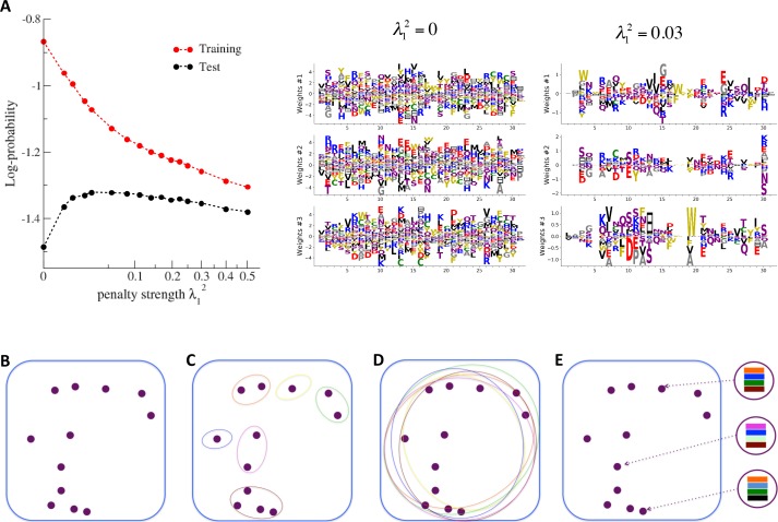
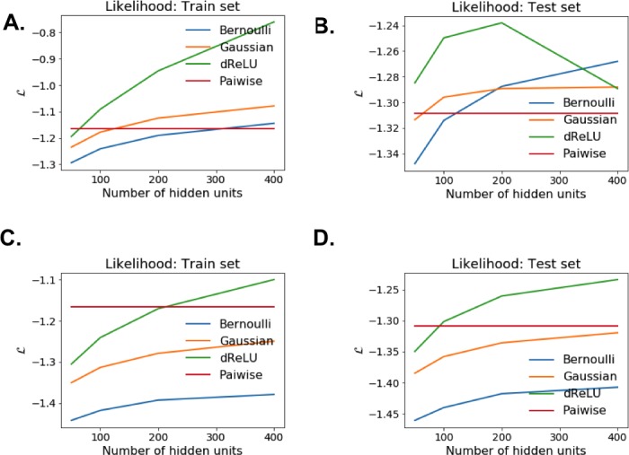
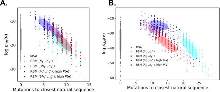
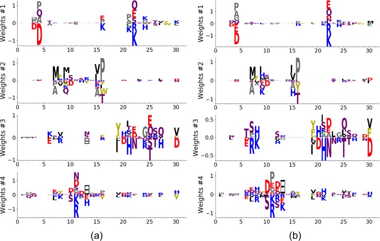
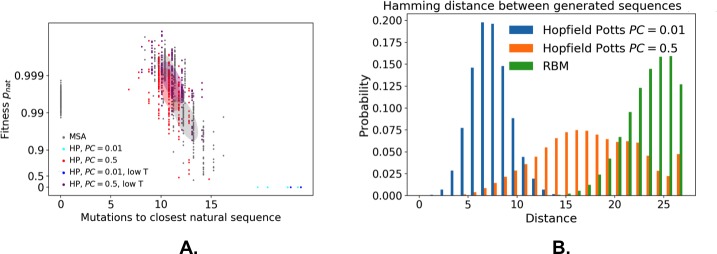
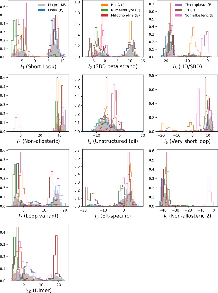
Statistical analysis of evolutionary-related protein sequences provides information about their structure, function, and history. We show that Restricted Boltzmann Machines (RBM), designed to learn complex high-dimensional data and their statistical features, can efficiently model protein families from sequence information. We here apply RBM to 20 protein families, and present detailed results for two short protein domains (Kunitz and WW), one long chaperone protein (Hsp70), and synthetic lattice proteins for benchmarking. The features inferred by the RBM are biologically interpretable: they are related to structure (residue-residue tertiary contacts, extended secondary motifs (α-helixes and β-sheets) and intrinsically disordered regions), to function (activity and ligand specificity), or to phylogenetic identity. In addition, we use RBM to design new protein sequences with putative properties by composing and 'turning up' or 'turning down' the different modes at will. Our work therefore shows that RBM are versatile and practical tools that can be used to unveil and exploit the genotype-phenotype relationship for protein families.

Keywords: coevolution; computational biology; machine learning; none; physics of living systems; sequence analysis; systems biology.

Figure 1.. Reverse and forward modeling of proteins.

(A) Example of Multiple-Sequence Alignment (MSA), here of the WW domain (PF00397). Each column $i=1,\mathrm{\dots },N$ corresponds to a site on the protein, and each line to a different sequence in the family. The color code for amino acids is as follows: red = negative charge (E,D), blue = positive charge (H, K, R), purple = non charged polar (hydrophilic) (N, T, S, Q), yellow = aromatic (F, W, Y), black = aliphatic hydrophobic (I, L, M, V), green = cysteine (C), grey = other, small amino acids (A, G, P). (B) In a Restricted Boltzmann Machine (RBM), weights $w_{i\mu }$ connect the visible layer (carrying protein sequences $\mathbf{𝐯}$) to the hidden layer (carrying representations $\mathbf{𝐡}$). Biases on the visible and hidden units are introduced by the local potentials $g_i(v_i)$ and ${𝒰}_{\mu }(h_{\mu })$. Owing to the bipartite nature of the weight graph, hidden units are conditionally independent given a visible configuration, and vice versa. (C) Sequences $\mathbf{𝐯}$ in the MSA (dots in sequence space, left) code for proteins with different phenotypes (dot colors). RBM define a probabilistic mapping from sequences $\mathbf{𝐯}$ onto the representation space $\mathbf{𝐡}$ (right), which is indicative of the phenotype of the corresponding protein and encoded in the conditional distribution $P(\mathbf{𝐡}|\mathbf{𝐯})$, Equation (3) (black arrow). The reverse mapping from representations to sequences is $P(\mathbf{𝐯}|\mathbf{𝐡})$, Equation (4) (black arrow). In turn, sampling a subspace in the representation space (colored domains) defines a complex subset of the sequence space, and allows the design of sequences with putative phenotypic properties that are either found in the MSA (green circled dots) or not encountered in Nature (arrow out of blue domain). (D) Three examples of potentials $𝒰$ defining the hidden-unit type in RBM (see Equation (1) and panel (B)): quadratic (black, $\gamma =0.2$, $\theta =0$) and double Rectified Linear Unit (dReLU) (dReLU1 (green), ${\gamma }_{+}={\gamma }_{-}=0.1$, ${\theta }_{+}=-{\theta }_{-}=1$; and dReLU2 (purple), ${\gamma }_{+}=1$, ${\gamma }_{-}=20$, ${\theta }_{+}=-6$, ${\theta }_{-}=25$) potentials. In practice, the parameters of the hidden unit potentials are fixed through learning of the sequence data. (E) Average activity of hidden unit $h$, calculated from Equation (3), as a function of the input $I$ defined in Equation (2). The three curves correspond to the three choices of potentials in panel (A). For the quadratic potential (black), the average activity is a linear function of $I$. For dReLU1 (green), small inputs $I$ barely activate the hidden unit, whereas dReLU2 (Purple) essentially binarizes the inputs $I$.

Figure 2.. Modeling Kunitz Domain with RBM.

(A) Sequence logo and secondary structure of the Kunitz domain (PF00014), showing two α-helices and two $\beta$-strands. Note the presence of the three C-C disulfide bridges between positions 11&35, 2&52 and 27&48. (B) Weight logos for five hidden units(see text). Positive and negative weights are shown by letters located, respectively, above and below the zero axis. Values of the norms ${\parallel W_{\mu }\parallel }_2=\sqrt{{\sum }_{i,v}{w}_{i\mu }{(v)}^2}$ are given. The color code for the amino acids is the same as that in Figure 1A. (C) Top: distribution of inputs $I_{\mu }(\mathbf{𝐯})$ over the sequences $\mathbf{𝐯}$ in the MSA (dark blue), and average activity vs. input function (full line, left scale); red points correspond to the activity levels used for design in Figure 5. Bottom: histograms of Hamming distances between sequences in the MSA (grey) and between the 20 sequences (light blue) with largest (for unit 2,3,4) or smallest (1,5) $I_{\mu }$. (D 3D visualization of the weights, shown on PDB structure 2knt Merigeau et al., 1998 using VMD Humphrey et al., 1996. White spheres denote the positions of the three disulfide bridges in the wildtype sequence. Green spheres locate residues $i$ such that ${\displaystyle \sum _v|w_{i\mu }(v)|>S}$, with $S=1.5$ for hidden units $\mu =1,2,3$, $S=1.25$ for $\mu =4$, and $S=0.5$ for $\mu =5$.

Figure 3.. Modeling the WW domain with RBM.

(A) Sequence logo and secondary structure of the WW domain (PF00397), which includes three $\beta$-strands. Note the two conserved W amino acids in positions 5 and 28. (B) Weight logos for four representative hidden units. (C) Corresponding inputs, average activities and distances between the top-20 feature-activating sequences. (D) 3D visualization of the features, shown on the PDB structure 1e0m Macias et al., 2000. White spheres locate the two W amino acids. Green spheres locate residues $i$ such that ${\displaystyle \sum _v|w_{i\mu }(v)|>0.7}$ for each hidden unit $\mu$. (E) Scatter plot of inputs $I_3$ vs. $I_4$. Gray dots represent the sequences in the MSA; they cluster into three main groups. Colored dots show artificial or natural sequences whose specificities, given in the legend, were tested experimentally. Upper triangle: natural, from Russ et al. (2005). Lower triangle: artificial, from Russ et al. (2005). Diamond: natural, from Otte et al. (2003). Crosses: YAP1 (0) and variants (1 and 2 mutations from YAP1), from Espanel and Sudol (1999). The three clusters match the standard ligand-type classification.

Figure 4.. Modeling HSP70 with RBM.

(A, B) 3D structures of the DNaK E. coli HSP70 protein in the ADP-bound (A: PDB: 2kho Bertelsen et al., 2009) and ATP-bound (B: PDB: 4jne Qi et al., 2013) conformations. The colored spheres show the sites carrying the largest entries in the weights in panel (C). (C) Weight logos for hidden units $\mu =1$, 2 and 5 (see Appendix 1—figure 21 for the other hidden units). Owing to the large protein length, we show only weights for positions $i$ with large weights (${\displaystyle \sum _v|w_{i\mu }(v)|>0.4\times \mathrm{m}\mathrm{a}{\mathrm{x}}_{\mathrm{i}}\sum _v|w_{i\mu }(v)|}$), with surrounding positions up to ±5 sites away; dashed lines vertical locate the left edges of the intervals. Protein backbone colors: blue = NBD; cyan = linker; red = SBD; gray = LID. Colors: orange = Unit 1 (NBD loop); black = Unit 2 (SBD β strand); green = Unit 3 (SBD/LID); yellow = Unit 4 (Allosteric). (D) Scatter plot of inputs $I_1$ vs. $I_2$. Gray dots represent the sequences in the MSA, and cluster into four main groups. Colored dots represent the main sequence categories based on gene phylogeny, function and expression. (E) Histogram of input $I_4$, showing separation between allosteric and non-allosteric protein sequences in the MSA.

Figure 5.. Sequence design with RBM.

(A) Conditional sampling of WW domain-modeling RBM. Sequences are drawn according to Equation (3), with activities $(h_3,h_4)$ fixed to $(h_4^{-},h_4^{+})$, $(h_3^{+},h_4^{-})$, $(h_3^{+},h_4^{+})$ and $(3h_3^{-},h_4^{-})$, see red points indicating the values of $h_3^{\pm },h_4^{\pm }$ in Figure 3C. Natural sequences in the MSA are shown with gray dots, and generated sequences with colored dots. Four clusters of sequences are obtained; the first three are putatively associated to, respectively, ligand-specific groups I, II/III and IV. The sequences in the bottom left cluster, obtained through very strong conditioning, do not resemble any of the natural sequences in the MSA; their binding specificity is unknown. (B) Sequence logo of the red sequences in panel (A), with ‘long ${\beta }_1$-${\beta }_2$ loop’ and ‘type I’ features. (C) Conditional sampling of Kunitz domain-modeling RBM, with activities $(h_2,h_5)$ fixed to $(h_2^{\pm },h_5^{\pm })$, see red dots indicating $h_2^{\pm },h_5^{\pm }$ in Figure 2C. Red sequences combine the absence of the 11–35 disulfide bridge and a strong activation of the Bikunin-AMBP feature, although these two phenotypes are never found together in natural sequences. (D) Sequence logo of the red sequences in panel (C), with ‘no disulfide bridge’ and ‘bikunin’ features. (E) Scatter plot of the number of mutations to the closest natural sequence vs log-probability, for natural (gray) and artificial (colored) WW domain sequences. The color code is the same as that in panel (A); dark dots were generated with the high-probability trick, based on duplicated RBM (see 'Materials and methods'). Note the existence of many high-probability artificial sequences far away from the natural ones. (F) The same scatter plot as in panel (E) for natural and artificial Kunitz-domain sequences.

Figure 6.. Contact predictions using RBM.

(A) Sketch of the derivation with RBM of effective epistatic interactions between residues. The change in log probability resulting from a double mutation (purple arrow) is compared to the sum of the changes accompanying the single mutations (blue and red arrows) (see text and 'Materials and methods', Equations (15,16)). (B) Positive Predictive Value (PPV) vs. pairs ${\displaystyle (i,j)}$ of residues, ranked according to their scores for the Kunitz domain. RBM predictions with quadratic (Gaussian RBM) and dReLU potentials are compared to direct coupling-based methods, namely the Pseudo-Likelihood Method (plmDCA) Ekeberg et al., 2014) and Boltzmann Machine (BM) learning Sutto et al., 2015). (C) Same as panel (B) for the WW domain. (D) Distant contact predictions for the 17 protein domains used to benchmark plmDCA in Ekeberg et al. (2014) obtained using fixed regularization ${\displaystyle {\lambda }_1^2=0.1}$ and ${\displaystyle M=0.3\times N\times 20}$. PPV for contacts between residues separated by at least five sites along the protein backbone vs. ranks of the corresponding couplings, expressed as fractions of the protein length ${\displaystyle N}$; solid lines indicate the median PPV and colored areas the corresponding 1/3 to 2/3 quantiles.

Figure 7.. Benchmarking RBM with lattice proteins.

(A) $S_A$, one of the 103,406 distinct structures that a 27-mer can adopt on the cubic lattice Shakhnovich and Gutin, 1990. Circled sites are related to the features shown in Figure 6C. (B)$S_G$, another fold with a contact map (set of neighbouring sites) close to $S_A$ Jacquin et al., 2016. (C) Four weight logos for a RBM inferred from sequences folding into $S_A$, see 'Supporting Information' for the remaining 96 weights. Weight 1 corresponds to the contact between sites 3 and 26, see black dashed contour in panel (A). The contact can be realized by amino acids of opposite (-+) charges (${\displaystyle I_1>0}$) or by hydrophobic residues (${\displaystyle I_1<0}$). Weights 2 and 3 are related to, respectively, the triplets of amino acids 8-15-27 and 2-16-25, each realizing two overlapping contacts on $S_A$ (blue dashed contours). Weight 4 codes for electrostatic contacts between sites 3 & 26, 1 & 18 and 1 & 20, and imposes the conditon that the charges of amino acids 1 and 26 have the same sign. The latter constraint is not due to the native fold (1 and 26 are ‘far away’ on $S_A$) but because folding must be impeded in the ‘competing’ structure, $S_G$ (Figure 7B and 'Materials and methods') in which sites 1 and 26 are neighbours Jacquin et al., 2016). (D) Distributions of inputs ($I$) and average activities (full line, left scale). All features are activated across the entire sequence space (not shown). (E) Conditional sampling with activities ${\displaystyle (h_2,h_3)}$ fixed to ${\displaystyle (h_2^{\pm },h_3^{\pm })}$, see red dots in panel (D). Designed sequences occupy specific clusters in the sequence space, corresponding to different realizations of the overlapping contacts encoded by weights 2 and 3 (Figure 6C). Conditioning to ${\displaystyle (h_2^{-},h_3^{+})}$ makes it possible to generate sequences combining features that are not found together in the MSA (see bottom left corner), even with very high probabilities (see 'Materials and methods'). (F) Scatter plot of the number of mutations to the closest natural sequence vs. the probability $p_{nat}$ of folding into structure ${\displaystyle S_A}$ (see Jacquin et al., 2016 for a precise definition) for natural (gray) and artificial (colored) sequences. Note the large diversity and the existence of sequences with higher ${\displaystyle p_{nat}}$ than those in the training sample.

Figure 8.. Nature of the representations built by RBM and interpretability of weights.

(A) The effect of sparsifying regularization. Left: log-probability (see , Equation (5)) as a function of the regularization strength ${\lambda }_1^2$ (square root scale) for RBM with $M=100$ hidden units trained on WW domain sequence data. Right: the weights attached to three representative hidden units are shown for ${\lambda }_1^2=0$ (no regularization) and 0.03 (optimal log-likelihood for the test set, see left panel); weights shown in Figure 3 were obtained at higher regularization ${\lambda }_1^2=0.25$. For larger regularization, too many weights vanish, and the log-likelihood diminishes. (B) Sequences (purple dots) in the MSA attached to a protein family define a highly sparse subset of the sequence space (symbolized by the blue square), from which a RBM model is inferred. The RBM then defines a distribution over the entire sequence space, with high scores for natural sequences and over many more other sequences putatively belonging to the protein family. The representations of the sequence space by RBM can be of different types, three examples of which are sketched in the following panels. (C) Mixture model: each hidden unit focuses on a specific region in sequence space (color ellipses, different colors correspond to different units), and the attached weights form a template for this region. The representation of a sequence thus involves one (or a few) strongly activated hidden units, while all remaining units are inactive. (D) Entangled model: all hidden units are moderatly active across the sequence space. The pattern of activities vary from one sequence to another in a complex manner. (E) Compositional model: a moderate number of hidden units are activated for each protein sequence, each recognizing one of the motifs (shown by colors) in the sequence and controling one of the protein's biological properties. Composing the different motifs in various ways (right circled compositions) generates a large diversity of sequences.

Figure 9.. Representative weights of the protein families selected in Ekeberg et al. (2014).

RBM parameters: ${\displaystyle {\lambda }_1^2=0.25}$, ${\displaystyle M=0.05\times N\times 20}$. The format is the same as that used in Figures 2B, 3B and 4B. Weights are ordered by similarity, from top to bottom: Sushi domain (PF00084), Heat shock protein Hsp20 (PF00011), SH3 Domain (PF00018), Homeodomain protein (PF00046), Zinc finger–C4 type (PF00105), Cyclic nucleotide-binding domain (PF00027), and RNA recognition motif (PF00076). Green spheres show the sites that carry the largest weights on the 3D folds (in order, PDB: 1elv, 2bol, 2hda, 2vi6, 1gdc, 3fhi, 1g2e). The ten weights with largest norms in each family are shown in Supplementary files 5–6.

Figure 10.. Representative weights of the protein families selected in Ekeberg et al. (2014).

RBM parameters: ${\lambda }_1^2=0.25$, $M=0.05\times N\times 20$. The format is the same as that used in Figures 2B, 3B and 4B. Weights are ordered by similarity (from top to bottom): SH2 domain (PF00017), superoxide dismutase (PF00081), K homology domain (PF00013), fibronectin type III domain (PF00041), double-stranded RNA-binding motif (PF00035), zinc-binding dehydrogenase (PF00107), cadherin (PF00028), glutathione S-transferase, C-terminal domain (PF00043), and 2Fe-2S iron-sulfur cluster binding domain (PF00111). Green spheres show the sites that carry the largest weights on the 3D folds (in order, PDB: 1o47, 3bfr, 1wvn, 1bqu, 1o0w, 1a71, 2o72, 6gsu, 1a70). The ten weights with largest norms in each family are shown in Supplementary files 5–6.

Figure 11.. Duplicate RBM for biasing sampling toward high-probability sequences.

Visible-unit configurations $\mathbf{𝐯}$ are sampled from ${\displaystyle P_2(\mathbf{v})\propto P(\mathbf{v}{)}^2}$.

Appendix 1—figure 1.. Model selection for RBM trained on the Lattice Proteins MSA.

Likelihood estimates for various potentials and number of hidden units, evaluated on train and held-out test sets. Top row: without regularization (${\lambda }_1^2=0$). Bottom row: with regularization (${\lambda }_1^2=0.025$).

Appendix 1—figure 2.. Model selection for RBM trained on the WW domain MSA.

Likelihood estimates for various potentials and number of hidden units, evaluated on train and held-out test sets. Top row: without regularization (${\lambda }_1^2=0$). Bottom row: with regularization (${\lambda }_1^2=0.25$).

Appendix 1—figure 3.. Sparsity-generative performance trade-off for RBM trained on the MSA of the Lattice Protein SA.

(A–D) Likelihood as function of regularization strength, for $L_1^2$ (top) and $L_1$ (bottom) sparse penalties, on train(left) and test (middle) sets. (E) Number $M_{eff}$ of connected hidden units (such that ${\max }_{i,v}|w_{i\mu }(v)|>0$) against effective strength penalty, for $L_1$ and $L_1^2$ penalties. For $L_1$ penalty, ${\lambda }_1^{eff}={\lambda }_1$; for $L_1^2$, ${\lambda }_1^{eff}={\lambda }_1^2\frac{1}{NMq}{\sum }_{\mu ,i,v}|w_{\mu i}(v)|$.

Appendix 1—figure 4.. Hidden layer representation redundancy as a function of the hidden-unit potentials.

Distribution of Pearson correlation coeffcients between hidden-unit average activities, for RBM trained with $M=100$, on (a) Lattice Proteins MSA, (b) Kunitz domain MSA, and (c) WW domain MSA. Bernoulli RBM feature the highest correlations.

Appendix 1—figure 5.. Comparison of Gaussian and dReLU RBM with M=100 trained on the Kunitz domain MSA.

Scatter plot of likelihoods for each model, where each point represents a sequence of the MSA. The color code is defined in Equation 19; hot colors indicate ’outlier’ sequences.

Appendix 1—figure 6.. Quantitative quality assessment of sequences generated by RBM trained on the Lattice Protein MSA.

(a) Distributions of the probability ${\displaystyle p_{nat}}$ of folding into the native structure $S_A$ (Equation (14) in 'Materials and methods'), for sequences generated by various models. The horizontal bars locate the average values of ${\displaystyle p_{\text{n}at}}$. Models with higher capacity (more parameters, less regularization) generate sequences with higher quality but lower diversity. (b) Distribution of distances from a randomly selected wildtype. The unregularized BM samples have lower diversity, whereas the regularized RBM samples better reproduce the data distribution. (c) Log-probability of dReLU RBM $M=100$ shown in the main text (Figure 7) vs true fitness evaluated on sequences from the MSA used (train) or not (test) for training.

Appendix 1—figure 7.. Quality assessment of sequences generated by RBM trained on (a) the Kunitz domain MSA and (b) the WW domain MSA.

Scatter plot of the number of mutations to the closest natural sequence vs log-probability of a BM trained on the same data, for natural (gray) and RBM-generated (colored) WW domain sequences. The color code is that same as that used in Figure 5A. Note similar likelihoods values for RBM-generated sequences and natural ones, including the unseen $(h_4^{-},h_5^{+})$ combinations.

Appendix 1—figure 8.. Evaluating the role of regularization and sequence reweighting on generated sequence diversity for the WW domain.

The y-axis indicates the log-likelihood of the data generated by the model; entropy is the negative average log-likelihood.

Appendix 1—figure 9.. Pairwise couplings learned from Kunitz domain MSA.

Scatter plot of inferred pairwise direct couplings learned by BM vs effective pairwise couplings computed from the RBM through Equation (15) in the 'Materials and methods'.

Appendix 1—figure 10.. Contact map and contact predictions for the Kunitz domain.

(a) Lower diagonal: the 551 pairs of residues at ${\displaystyle D<0.8}$ nm in the structure. Upper diagonal: top 551 contacts predicted by dReLU RBM with ${\displaystyle M=100}$, shown in Figure 2. (b) Positive Predicted Value vs rank for distant contacts ${\displaystyle |i-j|>4}$ for RBM (${\displaystyle M=100}$) and pairwise models. Distant contacts are well predicted, including those involved in the secondary structure.

Appendix 1—figure 11.. Contact predictions for Lattice Proteins, with (a) Bernoulli (b) Gaussian (c) dReLU RBM and (d) BM potentials.

Models with quadratic or dReLU potentials and large number of hidden units are typically similar in performance to pairwise models, trained either with Monte Carlo or Pseudo-likelihood Maximization.

Appendix 1—figure 12.. Contact predictions as a function of RBM parameters for (a) Kunitz and (b) WW domains.

Both panels show the area under curve metric (integrated up to the true number of contacts) for various trainings, with different training parameters, regularization choice and hidden units number/potentials, against the weight sparsity. In both cases, large sparse regularization and a high number of hidden units reproduce the performance of the pairwise models.

Appendix 1—figure 13.. Features inferred using the first and second half of the sequences.

Appendix 1—figure 14.. Top 12 patterns with highest contributions to the log-probability, see eqn (23) in Cocco et al. (2013), inferred by the Hopfield-Potts model on the Kunitz domain.

Appendix 1—figure 15.. Top 12 patterns with the highest contributions to the log-probability (see equation (23) in Cocco et al. (2013)), inferred by the Hopfield-Potts model on the WW domain.

Appendix 1—figure 16.. Top 12 patterns with the highest contributions to the log-probability (see equation (23) in Cocco et al. (2013), inferred by the Hopfield-Potts model on the Lattice Proteins data.

Appendix 1—figure 17.. Hopfield-Potts model for sequence generation.

(A) Fitness ${\displaystyle p_{\text{nat}}}$ against distance to closest sequence for the Hopfield-Potts model with pseudo-count 0.01 or 0.5, sampled with or without the high ${\displaystyle P(\mathbf{v})}$ bias. Gray ellipses denote the corresponding values for the RBM. (B) Distribution of distances between generated sequences.

Appendix 1—figure 18.. Contact prediction for 17 protein families including the Hopfield-Potts model.

Appendix 1—figure 19.. Phylogenetic identity of feature-activating Kunitz sequences with the RBM shown in Figure 2.

(A) Scatter plot of inputs of hidden units 2 and 3; color depicts the organisms' position in the phylogenic tree of species. Most of the sequences that lack the disulfide bridge are nematodes. (B) Sequence logo of the 137 sequences above the dashed line (${\displaystyle I_3>3}$), showing the electrostatic triangle that putatively replaces the disulfide bridge.

Appendix 1—figure 20.. Distribution of inputs for the five features shown in main text plus hidden unit 34.

Distributions of inputs for Kunitz domains belonging to specific genes are shown.

Appendix 1—figure 21.. Truncated weight logo of 10 selected HSP70 hidden units (1/2).

Appendix 1—figure 22.. Truncated weight logo of 10 selected HSP70 hidden units (2/2).

Appendix 1—figure 23.. Corresponding structures (1/3).

Left: ADP-bound conformation (PDB: 2kho). Right: ATP-bound conformation (PDB: 4jne). For the last hidden unit, we show the structure of the dimer Hsp70–Hsp70 in ATP conformation (PDB: 4JNE), highlighting dimeric contacts.

Appendix 1—figure 24.. Corresponding structures (2/3).

Left: ADP-bound conformation (PDB: 2kho). Right: ATP-bound conformation (PDB: 4jne). For the last hidden unit, we show the structure of the dimer Hsp70–Hsp70 in ATP conformation (PDB: 4JNE), highlighting dimeric contacts.

Appendix 1—figure 25.. Corresponding structures (3/3).

Left: ADP-bound conformation (PDB: 2kho). Right: ATP-bound conformation (PDB: 4jne). For the last hidden unit, we show the structure of the dimer Hsp70–Hsp70 in ATP conformation (PDB: 4JNE), highlighting dimeric contacts.

Appendix 1—figure 26.. Corresponding input distributions.

Note that both hidden unit 4 and 9 discriminate the non-allosteric subfamily from the rest; and that hidden unit 8 discriminates eukaryotic Hsp expressed in the endoplasmic reticulum from the rest.

Appendix 1—figure 27.. Some scatter plots of inputs for the 10 hidden units shown.

Appendix 1—figure 28.. Statistics of the length and amino-acid content of the unstructured tail of Hsp70.

Hidden unit 5 defines a set of sites, mostly located on the unstructured tail of Hsp70; its sequence logo and input distribution suggests that for a given sequence, the tail can be enriched either in tiny (A, G)or hydrophilic amino-acids (E,D,K,R,T,S,N,Q). This is qualitatively confirmed by the non-gaussian statistics of the distributions of the fractions of tiny and hydrophilic amino-acids in the tail (blue histograms and top left contour plots). This effect could, however, be due to the variable length of the loop (bottom histogram). To assess this enrichment, we built a null model where the tail size was random (same statistics as Hsp70), and each amino-acid was drawn randomly, independently from the others, using the same amino-acid frequency as that in the tail of Hsp70. The null model statistics (orange histograms and lower left contour plots) are clearly different, validating the collective mode.

References

1. Ackley DH, Hinton GE, Sejnowski TJ. Readings in Computer Vision. Elsevier; 1987. A learning algorithm for boltzmann machines; pp. 522–533.
1. Appel W. Chymotrypsin: molecular and catalytic properties. Clinical Biochemistry. 1986;19:317–322. doi: 10.1016/S0009-9120(86)80002-9. - DOI - PubMed
1. Ascenzi P, Bocedi A, Bolognesi M, Spallarossa A, Coletta M, De Cristofaro R, Menegatti E. The bovine basic pancreatic trypsin inhibitor (Kunitz inhibitor): a milestone protein. Current Protein & Peptide Science. 2003;4:231–251. doi: 10.2174/1389203033487180. - DOI - PubMed
1. Ashkenazy H, Abadi S, Martz E, Chay O, Mayrose I, Pupko T, Ben-Tal N. ConSurf 2016: an improved methodology to estimate and visualize evolutionary conservation in macromolecules. Nucleic Acids Research. 2016;44:W344–W350. doi: 10.1093/nar/gkw408. - DOI - PMC - PubMed
1. Bajaj MS, Birktoft JJ, Steer SA, Bajaj SP. Structure and biology of tissue factor pathway inhibitor. Thrombosis and Haemostasis. 2001;86:959–972. doi: 10.1055/s-0037-1616518. - DOI - PubMed
Publication types