Dynamic flood modeling essential to assess the coastal impacts of climate change

Abstract

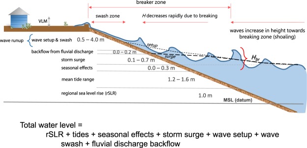
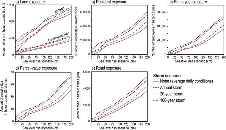
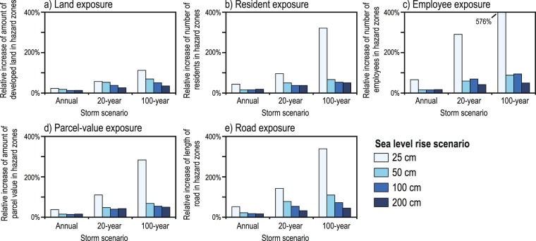
Coastal inundation due to sea level rise (SLR) is projected to displace hundreds of millions of people worldwide over the next century, creating significant economic, humanitarian, and national-security challenges. However, the majority of previous efforts to characterize potential coastal impacts of climate change have focused primarily on long-term SLR with a static tide level, and have not comprehensively accounted for dynamic physical drivers such as tidal non-linearity, storms, short-term climate variability, erosion response and consequent flooding responses. Here we present a dynamic modeling approach that estimates climate-driven changes in flood-hazard exposure by integrating the effects of SLR, tides, waves, storms, and coastal change (i.e. beach erosion and cliff retreat). We show that for California, USA, the world's 5^th largest economy, over $150 billion of property equating to more than 6% of the state's GDP and 600,000 people could be impacted by dynamic flooding by 2100; a three-fold increase in exposed population than if only SLR and a static coastline are considered. The potential for underestimating societal exposure to coastal flooding is greater for smaller SLR scenarios, up to a seven-fold increase in exposed population and economic interests when considering storm conditions in addition to SLR. These results highlight the importance of including climate-change driven dynamic coastal processes and impacts in both short-term hazard mitigation and long-term adaptation planning.

Figure 1

Dynamic water level concept. Example from California for 1 m of sea level rise of the significant water level components that comprise total water levels on a beach during a storm along the coast resulting in potential flooding. The range of values are based on observations and modeling conducted during the development and application of the Coastal Storm Modeling System (CoSMoS) across the region^,,. (VLM = vertical land motion, H = wave height, H_br = breaking wave height).

Figure 2

Coastal Storm Modeling System (CoSMoS) workflow. CoSMoS features a series of coupled numerical models that translates the physical forcing derived from Global Climate Models into local coastal flood projections, incorporating sea level rise, tides, seasonal effects, storm surge, fluvial discharge, and waves, as well as short- and long-term coastal change. The hybrid numerical-statistical model is used to develop continuous time-series of total water levels at the shore using a linear superposition of wave runup (maximum excursion that waves reach onshore), storm surge, and sea levels, in contrast to the numerically modeled flood maps which simulate non-linear interactions between changing water depths and waves. For more information on the CoSMoS framework see the Methods section and Supplementary Fig. 1. Figure modified from O’Neill et al.. Software citations: WaveWatch3 – v. 3.14, polar.ncep.noaa.gov/waves/wavewatch; Delft3D and SWAN – Delft3D v. 4.01, oss.deltares.nl/web/delft3d with Matlab v. 2015b (mathworks.com) and Global Mapper v. 17 (bluemarblegeo.com) used to generate images.

Figure 3

Study area and coastal flooding examples due to an extreme storm. (a) Study area for CoSMoS with insets. Examples of modeled flood extents for the 100-year coastal storm in combination with 0, 0.50, 1.00, 1.50, 2.00 and 5.00 m of SLR: (b) San Francisco International Airport, (c) City of Pacifica, (d) Port of Los Angeles and Port of Long Beach, (e) Port of San Diego and San Diego International Airport, and (f) City of Del Mar. (Figure generated using ArcGIS v. 10.4.2, www.esri.com. Local basemaps from http://services.arcgisonline.com/arcgis/services, World_Terrain_Base and ESRI_Imagery_World_2D, accessed 2 Oct 2018).

Figure 4

Examples of coastal flooding with 0.25 m of sea level rise and storms. These examples illustrate that there are locations with significant flood risks for small amounts of sea level rise when storms are considered. The left hand series of panels depicts projected coastal flood extent during average conditions (i.e. daily/background conditions with spring tide), and the right side select storm scenarios: (a) Santa Barbara Municipal Airport, (b) Alamitos Bay, Long Beach, and (c) Foster City. See Fig. 3 for locations. “Disconnected, low-lying flood hazard” designates areas that are below the flood elevation surface but are not hydraulically connected to the flooding due to a flow impediment (e.g. levee), and therefore subject to flooding should the flood barrier fail. See Supplementary Fig. 2 to see the uncertainty range for each of the scenarios. (Figure generated using ArcGIS v. 10.4.2, www.esri.com. Local basemaps from http://services.arcgisonline.com/arcgis/services, World_Terrain_Base and ESRI_Imagery_World_2D, accessed 2 Oct 2018).

Figure 5

Absolute changes in exposure to coastal-flooding hazards. Absolute changes in flooding exposure based on variations in sea level rise and storm scenarios for: (a) land, (b) residents, (c) employees, (d) parcel value, and (e) roads for the California study area. All values are in 2010 U.S. dollars.

Figure 6

Relative changes in exposure to coastal-flooding hazards. Relative changes in flooding exposure based on variations in sea level rise and storm scenarios for: (a) land, (b) residents, (c) employees, (d) parcel value, and (e) roads for the California study area. Percentages note relative increases in exposure due to the inclusion of storm conditions compared to hazard exposure based solely on select sea level rise scenarios (i.e. 0.25 m, 0.50 m, 1.00 m, and 2.00 m). These estimates are based on present-day socioeconomic and land use conditions, and do not account for future economic growth, coastal development patterns, climate change mitigation measures, etc.

References

1. Merkens J-L, Reimann L, Hinkel J, Vafeidis AT. Gridded population projections for the coastal zone under the Shared Socioeconomic Pathways. Global Planet. Change. 2016;145:57–66.
1. Dangendorf S, et al. Reassessment of 20th century global mean sea level rise. P. Natl. Acad. Sci. 2017;114:5946–5951. - PMC - PubMed
1. Kopp RE, et al. Probabilistic 21st and 22nd century sea-level projections at a global network of tide-gauge sites. Earth’s Future. 2014;2:383–406.
1. Le Bars D, Drijfhout S, de Vries H. A. high-end sea level rise probabilistic projection including rapid Antarctic ice sheet mass loss. Environ. Res. Lett. 2017;12:1–10.
1. Diaz DB. Estimating global damages from sea level rise with the Coastal Impact and Adaptation Model (CIAM) Climatic Change. 2016;137:143–156.
Publication types