Exploring the GDB-13 chemical space using deep generative models

Abstract

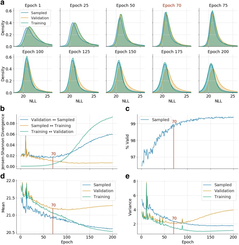
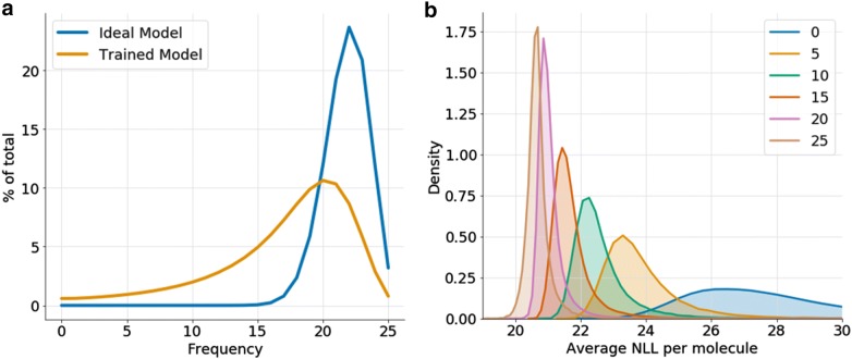
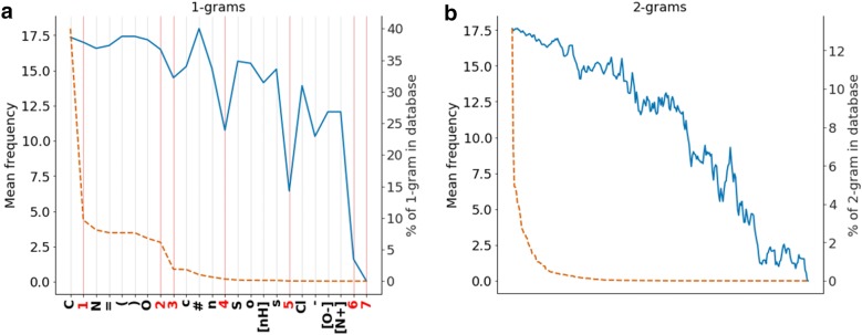
Recent applications of recurrent neural networks (RNN) enable training models that sample the chemical space. In this study we train RNN with molecular string representations (SMILES) with a subset of the enumerated database GDB-13 (975 million molecules). We show that a model trained with 1 million structures (0.1% of the database) reproduces 68.9% of the entire database after training, when sampling 2 billion molecules. We also developed a method to assess the quality of the training process using negative log-likelihood plots. Furthermore, we use a mathematical model based on the "coupon collector problem" that compares the trained model to an upper bound and thus we are able to quantify how much it has learned. We also suggest that this method can be used as a tool to benchmark the learning capabilities of any molecular generative model architecture. Additionally, an analysis of the generated chemical space was performed, which shows that, mostly due to the syntax of SMILES, complex molecules with many rings and heteroatoms are more difficult to sample.

Keywords: Chemical databases; Chemical space exploration; Deep generative models; Deep learning; Recurrent neural networks.

Fig. 1

Representation as an Euler diagram of the domain of a RNN trained with SMILES strings. The sets are the following, ordered by their size: All possible strings generated by an RNN (red), all possible valid SMILES (yellow), all possible SMILES of GDB-13 molecules (light blue), all canonical SMILES of GDB-13 molecules (dark blue) and the training set (black). Note that the relative sizes of the different subsets do not reflect their true size

Fig. 2

Example of a forward pass of nicotine (CN1CCCC1c1cccnc1) on a trained model. The symbol sampled from the probability distribution at the step $i$ (highlighted in black) is input at the step $i+1$. This, with the hidden state (h_i), enables the model to have time-dynamic behavior. Note that sometimes tokens with lower probability are sampled (like in step 1) due to the multinomial sampling of the model. Also note that the probability distributions are not from real trained models and that the vocabulary used throughout this publication is much bigger

Fig. 3

Metrics used to evaluate the training process. The red line at epoch 70 represents the chosen epoch used in further tests. The negative log-likelihood (NLL) is calculated with natural logarithms. a 10 NLL plots of the training, validation and sampled sets every 25 epochs (from 1 to 200) and the chosen epoch (70). b JSD plot between the three NLL distributions from the previous section for each of the 200 epochs. c Percentage of valid molecules in each epoch. Notice that the plot already starts at around 96.5%. Mean (d) and variance (e) of the three distributions from section (a). Note that spikes around epochs 1–20 are statistical fluctuations common in the beginning of the training process of a RNN, when the learning rate is high

Fig. 4

Results from sampling 2 billion SMILES from the 1 M model every five epochs (from 1 to 195). The red line at epoch 70 represents the chosen epoch for further tests. a Percent of the total sample (2B) that are valid SMILES, canonical SMILES, in GDB-13 and out of GDB-13. Solid lines represent all SMILES sampled, including repeats, whereas dotted lines represent only the unique molecules obtained from the whole count. b Close-up percentage of GDB-13 obtained every five epochs. Notice that the plot starts at around 54% and that the drop around epoch 10 correlates with the training fluctuations already mentioned in Fig. 3

Fig. 5

a Histograms of the frequency of the RNN models (orange) and the theoretical (binomial) frequency distribution of the ideal model (blue). b Histograms of the average NLL per molecule (from the 25 models) for molecules with frequency 0, 5, 10, 15, 20 and 25 computed from a sample of 5 million molecules from GDB-13

Fig. 6

a–f MQN PCA plots (Explained variance: $PC{A}_1=51.3\%,PC{A}_2=12,2\%$) calculated from a 130 million stratified sample of GDB-13 with 5 million molecules from each frequency value (0–25) colored by different descriptors. In all plots each pixel represents a group of similar molecules and its color represents the average value of a given descriptor. The colors rank from minimum to maximum: dark blue, cyan, green, yellow, orange, red and magenta. Each plot has the numeric range (min–max) between brackets after its title. Plots are colored by: a Number of trained models that generate each molecule. b Occupancy of every pixel. c Number of cyclic bonds. d Number of carbon atoms

Fig. 7

Plots of the frequency (left y axis) and the percent in database (right y axis) of 1 and 2-g in the canonical smiles of all GDB-13 molecules. The plot is sorted by the percentage present in the database. a Plot with the 1-g (tokens). In blue the mean frequency and in orange the percent of 1-g in database. Notice that the numeric tokens have been highlighted in red. b Plot with the 2-g mean frequency (blue) and percent (dashed orange). As the number of 2-g is too large (287), the x axis has been intentionally left blank and the mean frequency has been smoothed by an average window function size 8

Fig. 8

Distribution of a sample of 3 million molecules obtained from all the outside of GDB-13 sampled by the RNN model. a Histogram of the GDB-13 constraints broken by each molecule. Notice that a molecule can break more than one constraint. b Distribution of the number of GDB-13 constraints broken by each molecule