SEIS: Insight's Seismic Experiment for Internal Structure of Mars

Abstract

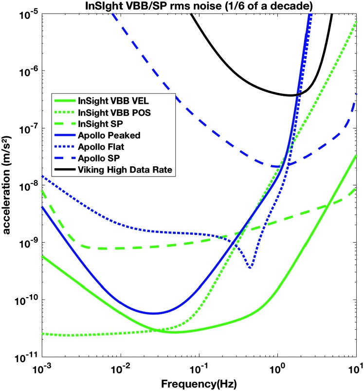
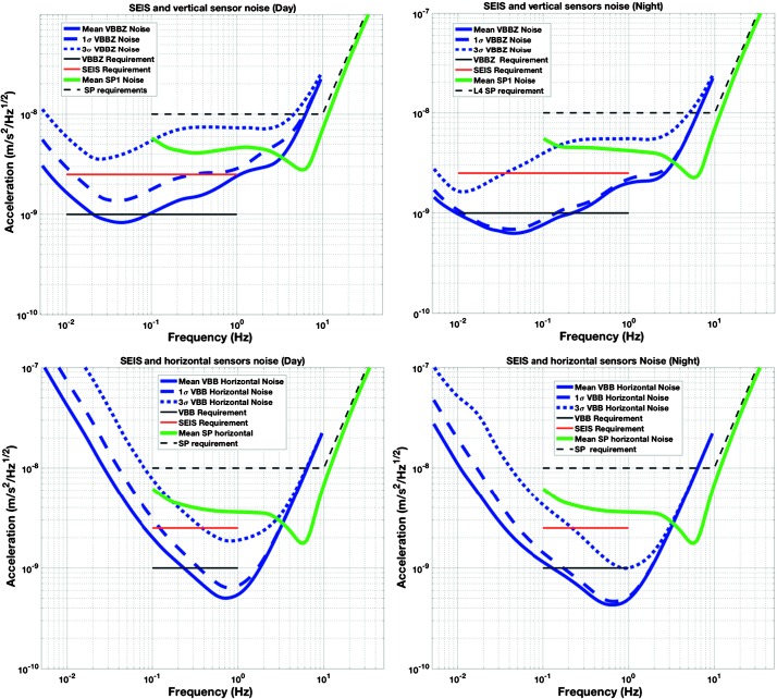
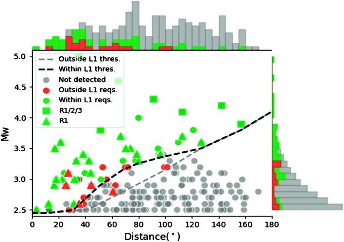
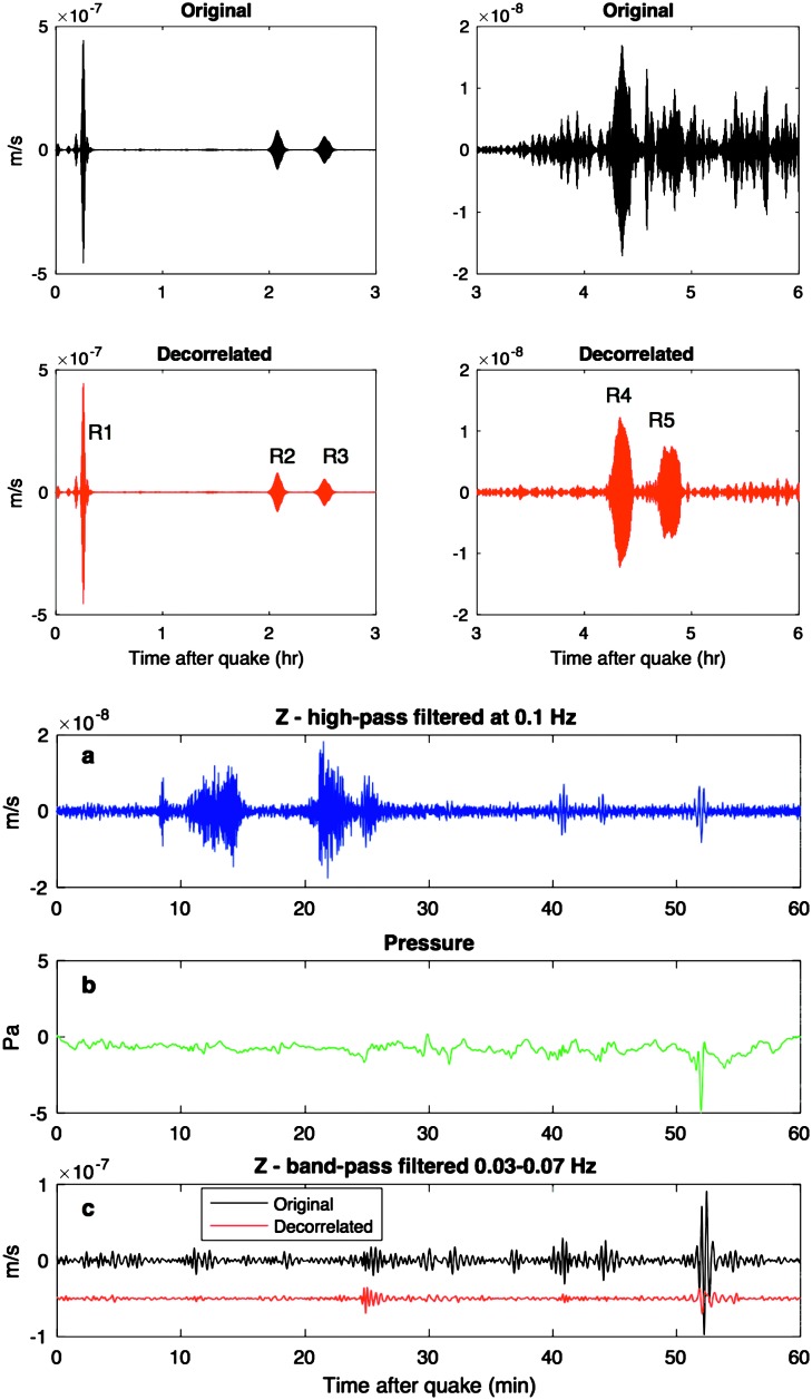
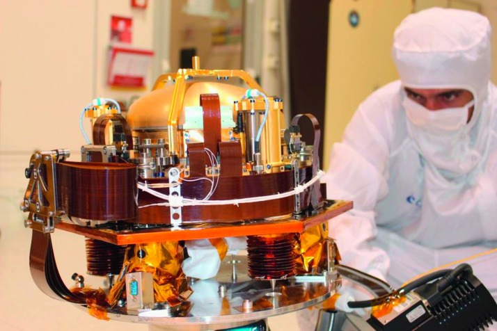
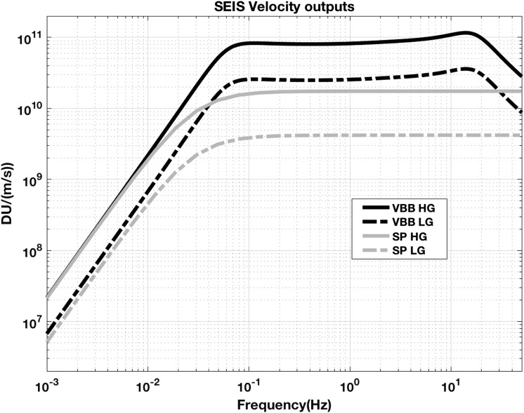
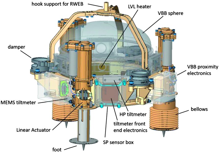
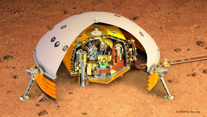
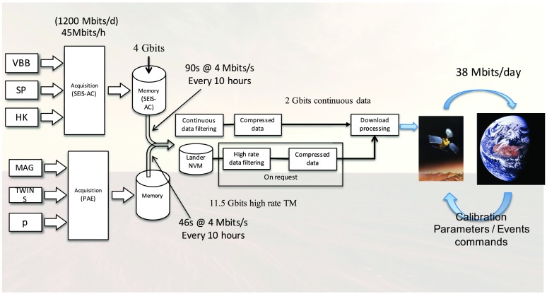
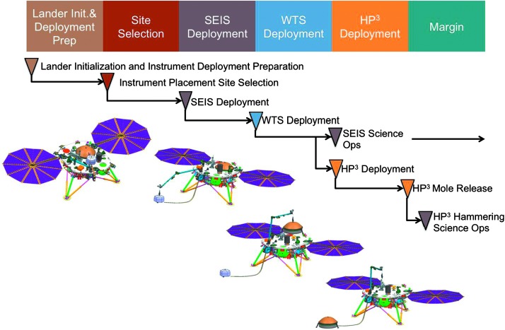
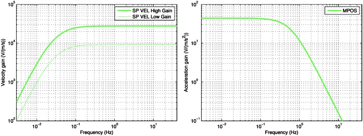
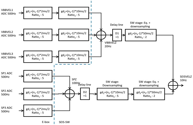
By the end of 2018, 42 years after the landing of the two Viking seismometers on Mars, InSight will deploy onto Mars' surface the SEIS (Seismic Experiment for Internal Structure) instrument; a six-axes seismometer equipped with both a long-period three-axes Very Broad Band (VBB) instrument and a three-axes short-period (SP) instrument. These six sensors will cover a broad range of the seismic bandwidth, from 0.01 Hz to 50 Hz, with possible extension to longer periods. Data will be transmitted in the form of three continuous VBB components at 2 sample per second (sps), an estimation of the short period energy content from the SP at 1 sps and a continuous compound VBB/SP vertical axis at 10 sps. The continuous streams will be augmented by requested event data with sample rates from 20 to 100 sps. SEIS will improve upon the existing resolution of Viking's Mars seismic monitoring by a factor of $\sim 2500$ at 1 Hz and $\sim 200000$ at 0.1 Hz. An additional major improvement is that, contrary to Viking, the seismometers will be deployed via a robotic arm directly onto Mars' surface and will be protected against temperature and wind by highly efficient thermal and wind shielding. Based on existing knowledge of Mars, it is reasonable to infer a moment magnitude detection threshold of $M_w\sim 3$ at ${40}^{\circ }$ epicentral distance and a potential to detect several tens of quakes and about five impacts per year. In this paper, we first describe the science goals of the experiment and the rationale used to define its requirements. We then provide a detailed description of the hardware, from the sensors to the deployment system and associated performance, including transfer functions of the seismic sensors and temperature sensors. We conclude by describing the experiment ground segment, including data processing services, outreach and education networks and provide a description of the format to be used for future data distribution.

Electronic supplementary material: The online version of this article (10.1007/s11214-018-0574-6) contains supplementary material, which is available to authorized users.

Keywords: InSight; Mars seismology.

Fig. 1

Sample suite of 13 models (color-coded as in legend in lower right). (A) $V_P$ (solid lines, in km/s), $V_S$ (dashed, in km/s) and density (dotted, in $\text{g}/{\text{cm}}^3$) as function of depth (km). (B) Shear quality factor ($Q$) as a function of depth. Models DWThot through EH45ThotCrust2b are from Rivoldini et al. (2011), ZG_DW is from Zharkov et al. (2009) and models DWAK through TAYAK are from Khan et al. (2018). Figure updated from Panning et al. (2017) with models available at: 10.5281/zenodo.1478804

Fig. 2

Body waves amplitude spectrum, for a 15 second window, as compared to the Earth Low Noise model (Peterson 1993) and for quakes of Moment ${10}^{15}\text{N}\text{m}$ at 45° (left) and 90° (right) of epicentral distance computed with a Gaussian beam method. The two dashed curves are for a shear Q_μ of 250 (upper curve) and 175 (lower curve) respectively in blue for P waves and red for S waves. On Earth, these body waves signals would be hidden by the micro-seismic peak. Note nevertheless the strong cutoff of amplitude at a few Hz, which shows that most for distant events amplitude will be recorded below 2 Hz for P body waves and below 1 Hz for S body waves

Fig. 3

Global stack of synthetic seismogram envelopes for a magnitude 4 (moment ${10}^{15}\text{N}\text{m}$) quake for two plausible Mars models, calculated using AxiSEM (Nissen-Meyer et al. ; van Driel et al. 2015). The seismograms were filtered with a noise-adapted filter suppressing all phases whose spectral power is below the noise level at all periods. In the plot, this corresponds to an amplitude of 0 dB. Note however, that phases with an amplitude of 0 dB can still be detectable, based on their polarization. Depth of the event is 10 km

Fig. 4

Normal mode summation synthetic seismograms for Mars shows large signals for multiple surface-wave arrivals from a ${10}^{16}\text{N}\text{m}$ quake at a distance of ${90}^{\circ }$ (5500 km). Filtering to isolate the Rayleigh waves suppresses the P and S arrivals around 10 minutes, which are actually quite strong ($\text{SNR}>70$ in a 0.1–1 Hz band). Black, green, purple and cyan traces are for source depths of 10, 20, 50 and 100 km, respectively. Red lines denote the RMS noise level for ${10}^{-9}\text{m}/{\text{s}}^2/{\text{Hz}}^{1/2}$ in amplitude spectral density in a bandwidth of 0.02–0.04 Hz, about $1.5\times {10}^{-10}\text{m}/\text{s}$. Dashed blue provide the amplitude model which was used in the requirement flow

Fig. 5

Root mean squared self-noise of the three main outputs of the SEIS instrument (VBB VEL, VBB POS and SP VEL), in acceleration for a $1/6$ of decade bandwidth, as a function of the central frequency of the bandwidth. This is compared to the Apollo and Viking resolution or LSB, as none of these instruments were able to record their self-noise due to limitations in the acquisition system for Apollo and Viking (9 bits plus sign for Apollo, 7 bits plus sign for Viking). SEIS uses acquisition at 23 bits plus sign

Fig. 6

Instrument noise. Vertical (top two figures) and horizontal noises (bottom two figures) for the day (left) and night (right) environmental conditions. Horizontal black and red lines represent the instrument performance requirements for the VBB self-noise and SEIS full noise (with environmental ones). Performances are presented for mean (50%), nominal $1\sigma$ (70%) and worst case $3\sigma$ (95%) conditions, respectively in dashed, dot-dashed and solid lines for the VBBs. Dashed black curve represents the SP sensor requirement while the green continuous line is the expected SP noise with environment for mean conditions. Curves are provided in the VBB and SP bandwidth, respectively [0.01–10 Hz] and [0.1–50 Hz]

Fig. 7

Summary of Marsquake Service performance in the Blind Test. All events included in the one year of data are shown. MQS detected the events shown in red and green, those in green meet L1 requirements. Squares indicate the events located using R1/R2/R3, triangles were located with R1 and circles are for only P and S waves. The grey curve indicates the limit threshold for detection and the black curve the location threshold, as a function of distance. See details in Clinton et al. (2018)

Fig. 8

Example of pressure decorrelation efficiency from synthetic tests following the techniques of Murdoch et al. (2017b). Event on the left is the one of the blind test data on 22/09/2019 and pressure decorrelation will enable much better long observations and therefore normal modes. The right example shows the R1 of a smaller quake on 27/03/2019. The bottom trace in black shows a clear detection of R1

Fig. 9

Deviation of the Phobos gravimetric factor l=2, m=2 (in red) and of the ratio between the $l=2$, $m=2$ and $l=4$, $m=4$ factors in blue. The second one varies by about $\pm 0.4\mathrm{\%}$ for the range of a-priori models but will not depend on an absolute calibration of SEIS

Fig. 10

SEIS experiment subsystems, together with the institutions leading the subsystems

Fig. 11

SEIS Sensor Assembly (SA) without the RWEB

Fig. 12

The Sensor Assembly being deployed on the ground during DST#3 (Deployment System Test). Two segments of the tether (TSA-1, part of TSA-), the Tether Storage Box, Field Joint and part of the Load Shunt Assembly are also visible

Fig. 13

Comparison of the VBBs and SPs transfer functions. Very long period gains are similar while the VBB gain is a factor of 4–5 times larger between 20 s and 10 Hz. All gains are in Digital Unit (DU) per ground velocity ($\text{m}/\text{s}$)

Fig. 14

Records of earthquakes detected by VBB14 (a) and VBB12 (b) in low gain engineering mode during temperature tests when located at IPGP (48.808°N 2.492°E): raw data (top), filtered data (middle) and spectrogram (bottom). (a) $M_w=7.8$ Solomon Islands earthquake occurred December 8, 2016, 17:38:46 UTC (epicenter location: 10.681°S 161.327°E, depth: 40 km, epicentral distance: 138.0°). The arrival times of PP and SS waves are indicated in red. P and S waves are not recorded at this epicentral distance. (b) $M_w=3.9$ earthquake occurred near Brest (France) December 11, 2016, 21:27:23 UTC (epicenter location: 48.490°N 4.460°W, depth: 2 km, epicentral distance: 4.6 km). Noise levels are all related to the test facility, a site very far from seismic vault conditions

Fig. 15

Record of local earthquake detected by QM SP1 in Acton, California: spectrogram (top), time series (bottom) for a $M_w=1.4$ ENE of Colton, California, occurred on July, 17th, 2016, 06:34:11 UTC. The time series show the full 80 Hz bandwidth from 200 sps (labeled SP), downsampled to the continuous stream of 2 sps (cont. SP) and using the energy in a 4 to 16 Hz filter downsampled to 2 sps (ESP)

Fig. 16

Record teleseismic earthquake detected by QM SP1 in Oxford UK: spectrogram of the incoherent noise with respect to the reference sensor, signal spectrogram (middle) and time series (bottom, for a reference seismometer, green, for the SP in blue with the difference in red) for a $M_w=7.7$, $29\text{km}$ SW of Agriha, Northern Mariana Islands at 2016-07-29 21:18:24 UTC. The red time signal is the one used for the coherence noise spectrogram

Fig. 17

15 degrees tilted configuration for extreme deployment conditions. As a low rigidity regolith is expected at surface, SEIS will however be always in contact with the flat disks of the three feet, in the center of which a spike will penetrate in the ground. The surface will therefore be deformed just beneath each foot

Fig. 18

LVL design as well as location of all sensor assembly subsystems

Fig. 19

The SEIS EBox. A $\sim 5\text{kg}$ and $\sim 9\text{W}$ electronic box. The E-box is 243.8 mm in height. The top is $303.5\text{mm}\times 125.5\text{mm}$ while the bottom is $343.5\text{mm}\times 169.5\text{mm}$ due to mounting structures

Fig. 20

The EBox and its electronic boards. The E-box is 243.8 mm in height. The top is $303.5\text{mm}\times 125.5\text{mm}$ while the bottom is $343.5\text{mm}\times 169.5\text{mm}$ due to mounting structures

Fig. 21

Tether System overview, Stowed Configuration. The Ebox is inside the Thermal Enclosure of the Lander. The Thermal Enclosure is not shown. The height of the Sensor Assembly on the InSight deck is about 33 mm and the distance from the center of the Sensor Assembly to the field joint is about the same

Fig. 22

Illustration of the RWEB and WTS configuration after deployment

Fig. 23

Cradle subsystem overview

Fig. 24

Sensor Assembly integration summary. Each VBB (a) is integrated in the crown (b). (c) Shells are welded on the crown, the vacuum is made and the exhaust tube (queusot) is pinched off. (d) VBBs can then be tested when connected to their PE (Proximity Electronics), one PE for each VBB. (e) The sphere and then all SPs (Short Period) are added to the LVL ring. (f) The cradle makes the mechanical link between the instrument and the lander. (g) The tether makes the electrical link between all the Sensor Assembly’s components and the Lander. (h) The RWEB provides a first protection, mainly thermal. (i) The WTS (Wind and Thermal Shield) is placed on the Sensor Assembly after the SA is deployed

Fig. 25

Transmission strategy of the SEIS experiment

Fig. 26

Deployment process of the SEIS experiment following the landing and prior to the HP3. This does not detail the deployment internal to the SEIS sensor assembly after Sensor Assembly deployment on the ground

Fig. 27

This figure presents the online tool developed by JPL/Caltech to evaluate and compare the performance of tentative deployment sites. The lander is represented in the lower part of the figure. Tentative positions for SEIS (pentagon) and WTS (circle) are figured on the top. The color code goes from blue to red. It represents the percentage of budget allocation for the wind noise on the overall instrument (red equal or superior to 100, deep blue zero percent of the allocation) for the 100 mHz horizontal noise

Fig. 28

Details of the 4 Frangibolt firings actions, each of them an irreversible action associated with locking systems. Respectively, these are (top left) the locking system of the SEIS SA on the deck, (top right) the Tether box opening for mechanical decoupling of the tether from the lander, (bottom left) the LSA opening for mechanical decoupling of the tether from the SEIS SA and (bottom right) the locking system of the Wind Shield

Fig. 29

SEIS Deployment (left) and grapple release (right)

Fig. 30

The closed tether box (left) is opened to release the tether onto the surface (right)

Fig. 31

Opening the Load Shunt Assembly (LSA) on the tether. The LSA mechanically decouples the seismometer from thermoelastic expansion and contraction of the tether

Fig. 32

The final stage in SEIS deployment is the placement of the WTS over the sensor assembly

Fig. 33

VBBs subsystem overview. It is composed of 3 sensors enclosed in the Evacuated Container (EC), 3 proximity electronics boxes hosted on the LVL and 3 feedback boards located into the E-box. The Tether provides the electrical connection between the feedback board and the PE

Fig. 34

The 3 VBB sensors in the spherical evacuated container (right) which has an outside diameter of 198 mm. Their three sensing directions form the tetrahedron shown on the left

Fig. 35

Inverted Pendulum Principle Schematic

Fig. 36

Picture of the pivot of VBB1, including electrical connections. The length of the pivot is 54 mm

Fig. 37

(a) One of the VBB sensor with Earth mass and VBB pendulum CAD views, illustrating the different functions of the sensor, (b) the fixed part, (c) the moving part, (d) the pivot, see Fig. 36, (e) the displacement Transducer, see Sect. 5.1.4, (f) the Feedback coils, see Sect. 5.1.5, (g) the re-centering motors, see Sect. 5.1.6 and Fig. 44, (h) the Thermal Compensation System, Sect. 5.1.8 and Fig. 45. A VBB pendulum fits in a $65\times 100\times 108{\text{mm}}^3$ volume

Fig. 38

All Flight and spare VBBs prior to the cherry-pick process which lead to the selection of the 3 Flight and the 3 spare units. Each VBB pendulum fits in a $65\times 100\times 108{\text{mm}}^3$ volume

Fig. 39

$Q$ of VBB 13 as a function of pressure. The gas in the chamber was air

Fig. 40

DCS noise. Nominal noise in red and VBB11 measurement in other colors. Noise above 1 Hz is residual micro-seismic background

Fig. 41

FB schematics. Top: ENG mode. Bottom: SCI mode

Fig. 42

FB transfer function at $-{55}^{\circ }\text{C}$ for unit VBB10. On left are the Transfer functions for the ground velocity and at right are those for the ground acceleration, in Digital Unit (DU) per ground velocity ($\text{m}/\text{s}$) or ground acceleration ($\text{m}/{\text{s}}^2$)

Fig. 43

Saturation Levels at $-{55}^{\circ }\text{C}$ for unit VBB10. Left are those of the SCI output and right those of the ENG outputs. In addition to the saturation of the outputs gains, the internal saturation is shown in red. In SCI mode, this internal saturation occurs at long period at the output of the INT2 filter and above about 1 Hz at the output of the displacement transducer. This internal saturation matches therefore the Low Gain modes of the instruments at long periods for POS LG and at short periods for VEL LG. The same is valid for the ENG, where the internal saturation is then only due to the displacement transducer saturation and matches the one of the POS LG output

Fig. 44

Re-centering mechanism from the top and from the side. A lead screw is driven by a stepper motor through a 1:256 gear box and a flex coupling to displace the mechanism. Two parallel guides prevent the motor gear box to rotate. To minimize overall mass, the motor is on the moving part. The re-centering mechanism fits in a $86\times 36\times 22{\text{mm}}^3$ volume. The motor and gear box have a 10 mm diameter

Fig. 45

Thermal Compensator Device Mechanism. Two thermal compensation devices are mounted on a shaft. A tuning mechanism allows tuning of their orientation in a vertical plane. It is composed of a stepper motor, a 1:256 gear box and a worm screw. The compensation device is $37\text{mm}\times 37.1\text{mm}$ and can extend $12\mathrm{\mu }\text{m}$ per °C. The orientation mechanism is 43.2 mm long. Its motor and gear box are 8 mm in diameter

Fig. 46

Thermal tests of one of the Flight VBBs (VBB3) during which the temperature of the VBB went from $-{70}^{\circ }\text{C}$ to $-{10}^{\circ }\text{C}$. The test was made on the POS ENG low gain (about $1500\text{V}{\text{s}}^2/\text{m}$), which has about 8 times less gain than the POS SCI low gain. In the neutral position (magenta solid line), signal varies by about 0.5 Volt from $-{52}^{\circ }\text{C}$ to $-9^{\circ }\text{C}$. On the right, dotted, long dashed and continuous red lines are for $\pm 5\times {10}^{-5}\text{m}/{\text{s}}^2/\text{K}$, $\pm 2\times {10}^{-5}\text{m}/{\text{s}}^2/\text{K}$ and $\pm 5\times {10}^{-6}\text{m}/{\text{s}}^2/\text{K}$ thermal sensitivities. Blue line corresponds to data measured during passive heating of the VBB. Left is for signal output in Volt while right is the temperature derivative, for a fixed gain and for the temperature sensitive gain. Black dotted lines are for the different positions of the TCDM. The very large temperature sensitivity at $-{60}^{\circ }\text{C}$ is suspected to be exaggerated by the testing device on Earth

Fig. 47

VBB 1 & 2 Thermal Sensitivity performances. VBB2 has higher thermal sensitivity at cold that exceed TCDM capabilities at low temperature. VBB2 meets its requirements over $-{55}^{\circ }\text{C}$. VBB1 is compliant over the full range. Color and lines definitions are the same as the right Fig. 46. Only the active tests results are shown for VBB2

Fig. 48

The unmounted SP sensors showing in (a) the top view of SP1, the vertical axis sensor and (b) the back view of SP2, one of the two horizontal axes

Fig. 49

The SP sensor mounted on its frame and connected to the proximity electronics

Fig. 50

The SP sensor assembly with the magnetic assembly and proximity electronics mounted on the SP sensor enclosure base prior to sealing

Fig. 51

A sealed horizontal SP unit viewed from (a) the connector side and (b) the LVL mounting direction

Fig. 52

A schematic of the SP electronics. SEIS-SC, the SEIS acquisition electronics are installed in the Ebox of the lander while the SP sensors are deployed on the Martian surface on the SEIS instrument assembly

Fig. 53

Solid lines: Generic shape of the Transfer functions of the SPs for the VEL output (left) and for the MPOS output (right). On the left, the dashed line is the low gain VEL output. The Full Scale Range of SEIS-AC is 25 Volt for SP VEL (with 24 bits) and 10 Volt for SP POS (with 12 bits for A/D and 16 bits after averaging)

Fig. 54

Linear guidance of the telescopic leg. The diameter of the telescopic length is 25 mm

Fig. 55

Geartrain of the linear actuator. The diameter of the telescopic legs is 25 mm

Fig. 56

MDE block diagram

Fig. 57

The place of the E-Box in the system

Fig. 58

The SEIS-AC acquisition electronics including redundancy

Fig. 59

Digital filtering in acquisition chain for velocity signals

Fig. 60

Digital filtering in acquisition chain for position and SCIT signals

Fig. 61

The reduction of gain error by offset compensation for temperatures

Fig. 62

The structure of packets containing seismic or housekeeping data

Fig. 63

The circular buffer as used for seismic and housekeeping data

Fig. 64

The acquisition noise breakdown of VBB VEL channels ($\text{FSR}=\pm 25\text{V}$, $1\text{LSB}=3\mathrm{\mu }\text{V}$)

Fig. 65

Tether System overview, Deployed Configuration. The TSA-3 and TSA-4 between the Tether Storage Box and the Ebox are unchanged from. The distance from the center of the Sensor Assembly of SEIS and the point below the Tether Storage Box is about 1.40 m in this configuration

Fig. 66

Construction and thicknesses of Tether belts

Fig. 67

Finite element mesh configuration for thermal and elastic models of the tether

Fig. 68

EC (Evacuated Container) with non-flight ground handling ring. The diameter of the sphere is 198 mm

Fig. 69

SEIS RWEB (Remote Warm Enclosure Box). The width of the RWEB is $\sim 355\text{mm}$ and its height is 212.5 mm

Fig. 70

SEIS WTS (Wind and Thermal Shield). It is 72 cm in diameter and 35 cm tall

Fig. 71

(Left) 37-pin and 2-pin electrical feedthrough installed into EC Crown; (Right) 37-pin feedthrough closeup

Fig. 72

Pinched-off queusot

Fig. 73

Sphere heat flow diagram under beginning of life pressure conditions. The average temperature in Celsius are given for the different units

Fig. 74

Cradle Dampers (on left) and internal design of the cradles with the release mechanism (on right). The cradles are 185.5 mm height

Fig. 75

Cradle damping efficiency. The left figure provides the damping of launch vibration, while the right figure provides the damping efficiency during cradle release. Red lines are those on the deck and blue lines are the acceleration levels at the SEIS assembly

Fig. 76

Typical setup with 5 reference seismometers. STS-2 BFO was covered by an air lock, STS-2 CNRS was covered by mu-metal/thermal shield and STS-2.5 only by thermal shield. SEIS was tilted at 68° to balance one VBB and the vertical SP

Fig. 77

Left: Big thermal shield used for tests. Right: Aluminum plate and goniometer mounting. SEIS was mounted on the goniometer while the reference seismometers were installed on the plate or nearby

Fig. 78

References sensors and reference acquisition systems used for the performance tests. From left to right, STS-2 and Trillium compact seismometers from Streckeisen and Nanometrics respectively, Q330HR and Centaur digitizers from Kinemetrics and Nanometrics respectively

Fig. 79

Typical setup with 5 reference seismometers. SEIS (not seen) is connected to the Ebox

Fig. 80

Setup for SEIS QM test in the Black Forest Observatory mine seismic vault. EBOX on the left, sensor assembly with “cuvinette” on the right. Once the tent was closed the reference seismometers were installed on the pillar in the foreground

Fig. 81

Top left: VBB in Earth configuration. The Earth mass is indicated by a black arrow. VBBs can operate in Earth mass in the nominal configuration but with a gain smaller than the Flight model by about 2.65. Top right. Flight model during tests as fixed on the test goniometer. The test goniometer was used to tilt the Sensor Assembly to the required position. Bottom left: one of the 68° positions, used for testing the VBB1. The rotation is made with a rotation axis in the direction of Y. During this rotation, both VBB1 and the vertical SP1 can be desaturated. Generally, fine recentering was made with the goniometer in order to reduce the use of the Flight unit’s recentering motors. Bottom right: Configuration for the 32° test, in which two VBBs as well as a horizontal SP can be desaturated and tested

Fig. 82

Details of the Transfer function between 30 s (0.03 Hz) and 30 Hz for the VEL output for the different testing configurations. Up to 30% of variations of the Transfer function are observed mostly due to the VBB frequency change. Gain is always larger than the 68° configuration which is close to the Flight configuration. Note however that even in this case, the pivot is operating in off-nominal condition, with a large force along its rotation axis due to the projected weight of the pendulum

Fig. 83

Modeling of the VBB seismometer output from a sweep calibration experiment. The top panel shows the current flowing through the calibration coil. It covers frequencies from 1 Hz to 0.01 Hz. The middle panel shows the output of the seismometer overlain with the modeled output and the residue, that is the difference between the two signals. The bottom panel shows only the residue. The modeled output fits the measured output so well that nothing from the sweep is visible in the residue. Only the background noise level from CNES is visible. Instrument parameters can be constrained more tightly if such test can be conducted at seismically quieter locations

Fig. 84

Dispersion of the gain measurements of the VBBs during coil calibration. Dispersions were ranging 4–6% for the VEL gain and 0.7–0.9% for the POS gain

Fig. 85

SEIS VBBs eigenfrequencies with respect to Temperature

Fig. 86

SEIS VBBs Magnetic actuators ratios of the force coefficient by the internal resistance with respect to Temperature. Coil A, B, C are the integrator, derivator and calibration coils respectively (see Sect. 5.1.5). Measurement errors remain large

Fig. 87

SEIS VBBs Theoretical VBBs Amplitude Response variation wrt Sphere Temperature from feedback actuator thermal sensitivity measurements. At periods larger than 100 s, the transfer function sensitivity is $<0.05\mathrm{\%}/{}^{\circ }\text{C}$, leading to 2.5% over the 50°C climatic variation between the coldest and hottest temperature of the VBBs over one Martian year

Fig. 88

SEIS POS output at the Phobos Tide frequency and SEIS VEL output at 100 s, as a function of temperature. Temperature dependency will be recalibrated on Mars but can be considered as linear as a function of frequency and with a frequency dependency as indicated by Fig. 85. The information of temperature dependency will be encrypted in a SEED comment

Fig. 89

Noise model of one VBB axis in Mars conditions, for Night and Day conditions, for both the VEL (left) HG and POS (right) HG. For LG, the acquisition noise will be respectively 3.2 and 4.5 larger for VEL and POS output respectively

Fig. 90

Results of tests made on the flight units in the CNES clean room, for both the POS and VEL outputs. The yellow curve shows the noise between two STS-2, which is significantly above the VBB noise model. The dashed green continuous curve is the VBB noise model while the continuous green curve is the quadratic sum between the VBB self-noise and the observed STS-2 noise, which might be more representative to the noise of the VBB with respect to a STS-2. Some of the VBBs measurements are very close to the environmental limits, despite the lower quality installation of the VBBs on the goniometer compared to the better installation quality of the STS-2

Fig. 91

Noise measurement of the VBB in Earth configuration at BFO

Fig. 92

Comparison of three closely colocated STS-2s at BFO

Fig. 93

Spectrogram of the VBB output in ground acceleration, during 10 hours of BFO tests with Earth configuration. The series of events seen at frequencies smaller than 0.01 Hz are likely related to pressure transient variations associated with the leak rate of the vacuum chamber used for the test and whose spectrum might be proportional to $f^{-1}$. The amplitudes shall be compared to those recorded by the STS-2s shown on Fig. 91

Fig. 94

The transfer function (TF) of SP determined from coherence testing shown in amplitude and phase. The requirement of $\pm 5\text{dB}$ flatness within the bandwidth of SP is shown. The TF determination is valid within the bandwidth where the coherence is high, allowing extension of SP meeting the TF requirements to 0.006 Hz

Fig. 95

Self noise of the flight model (FM) SP’s as determined by coherence testing on the SEIS instrument assembly at CNES Toulouse, together with the self-noise of a qualification model (QM) unit determined at the lower noise Black Forest Observatory (BFO). The SP performance requirement is marked as well as the noise models for the FM and QM units. All SPs are at least a factor of 2 better than their requirements at 0.1 Hz

Fig. 96

Position of SCIT A&B on the LVL subsystem

Fig. 97

HRTS-5760-B-U-0-12 sensor head

Fig. 98

Dry Heat chamber

Fig. 99

Location of MEMS (1) and HP tiltmeters (2) on the LVL

Fig. 100

SH 50055 Family Sensor

Fig. 101

Working principle of the HP sensors

Fig. 102

Temperature calibration curves for HP tiltmeter, measured at −20°C to 40°C in 20°C steps as described in the text

Fig. 103

Temperature calibration curves for MEMS tiltmeter, measured at −20°C to 40°C in 20°C steps as described in the text

Fig. 104

Measured (blue) and modeled (red) gain of the horizontal transfer functions in the LVL baseline configuration (all legs extended by 0.5 mm). Masses, leg lengths and values of $k_h^p$ of the model were set to those of the measurement, whereas parameters $k_h^g$, $C_h^g$ and $Q$ were adjusted to fit the data

Fig. 105

Schematic of the SEIS sensor assembly environment

Fig. 106

Views of the SA coatings

Fig. 107

Results of CFD computation on WTS in cold case with $20\text{m}/\text{s}$ wind

Fig. 108

Photos of TVAC#4 configuration

Fig. 109

TVAC#4 profile as realized

Fig. 110

Comparison data vs. temperature calculated with 1st order filter

Fig. 111

Comparison model-test data on the warm-up phase of Landed TVAC

Fig. 112

SEIS temperatures on Mars in cold operating case. Time is in Mars hours

Fig. 113

SEIS temperatures on Mars in hot operating case. Time is in Mars hours

Fig. 114

Air circulation impacting heat exchanges

Fig. 115

Overview of the SEIS Operations

Fig. 116

Event Request Selection Process

Fig. 117

Example of SEISVELZ production chain by Ebox (on the left side of blue dashed line) and FSW (on the right side of blue dashed line) from SP and VBB channels. The final product (SEISVELZ at 10 sps) is provided in the continuous data flow

Fig. 118

SISMOC functions with the roles of JPL (in red), CNES (in blue) and the Science services and team (in yellow)

Fig. 119

This summarizes the SEIS data flow from SISMOC to the scientific community

Fig. 120

Examples of preliminary demonstrations of the anticipated products of the MSS from Panning et al. (2017). (A) Example demonstration of the probability density function output for the Bayesian inversion of a small number of P, S and Rayleigh wave group arrival times for resolution of Earth mantle velocity structure. (B) A range of models of shallow crustal structure with color of plotting representing data misfit inverted to match synthetic Mars observations of the frequency dependent ratio of vertical component to horizontal component amplitude. (C) Bayesian inversion of mantle structure from noisy synthetic long period normal mode spectra. Green colors represent higher probability models while blue color is lower probability

Fig. 121

Data flow with key contact persons

Fig. 122

Seed volumes organization

Fig. 123

Hex dump of the station of cola.iu.liss.org. The most important fields are specified and linked to a description Table

References

1. H. Abarca, R. Deen et al., Image and data processing for InSight lander operations and science. Space Sci. Rev. (2018 this issue)
1. Ackerley N. Principles of broadband seismometry. In: Beer M., Kougioumtzoglou I.A., Patelli E., Siu-Kui Au I., editors. Encyclopedia of Earthquake Engineering. Berlin: Springer; 2014.
1. Agnew D.C. History of seismology. Int. Geophys. Ser. 2002;81:3–11. doi: 10.1016/S0074-6142(02)80203-0. - DOI
1. Anderson D.L., Given J. Absorption band Q model for the Earth. J. Geophys. Res. 1982;87:3893–3904. doi: 10.1029/JB087iB05p03893. - DOI
1. Anderson D.L., Miller W.F., Latham G.V., Nakamura Y., Toksoz M.N., Dainty A.M., Duennebier F.K., Lazarewicz A.R., Kowach R.L., Knight T.C. Seismology on Mars. J. Geophys. Res. 1977;82:4524–4546. doi: 10.1029/JS082i028p04524. - DOI