Multicompartment Magnetic Resonance Fingerprinting

Abstract

Magnetic resonance fingerprinting (MRF) is a technique for quantitative estimation of spin- relaxation parameters from magnetic-resonance data. Most current MRF approaches assume that only one tissue is present in each voxel, which neglects intravoxel structure, and may lead to artifacts in the recovered parameter maps at boundaries between tissues. In this work, we propose a multicompartment MRF model that accounts for the presence of multiple tissues per voxel. The model is fit to the data by iteratively solving a sparse linear inverse problem at each voxel, in order to express the measured magnetization signal as a linear combination of a few elements in a precomputed fingerprint dictionary. Thresholding-based methods commonly used for sparse recovery and compressed sensing do not perform well in this setting due to the high local coherence of the dictionary. Instead, we solve this challenging sparse-recovery problem by applying reweighted-𝓁₁-norm regularization, implemented using an efficient interior-point method. The proposed approach is validated with simulated data at different noise levels and undersampling factors, as well as with a controlled phantom-imaging experiment on a clinical magnetic-resonance system.

Keywords: Quantitative MRI; coherent dictionaries; magnetic resonance fingerprinting; multicompartment models; parameter estimation; reweighted 𝓁1 -norm; sparse recovery.

Figure 1:

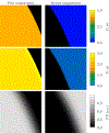
MRF reconstruction of a sharp boundary between two tissue regions with constant proton density (PD) and relaxation times corresponding to gray matter (T₁ = 1123 ms, T₂ = 88 ms) and cerebrospinal fluid (T₁ = 4200 ms, T₂ = 2100 ms) [29]. Due to the limited resolution caused by the low-pass measurements depicted by a red rectangle in the image at the center, voxels close to the boundary contain signals from the two tissues. This leads to erroneous parameter estimations near the boundary when using the standard MRF single-compartment reconstruction. A multicompartment model would be required to identify the correct relaxation times of the two contributing compartments.

Figure 2:

The left image shows the simulated signals corresponding to two different tissues: intra/extra (I/E) axonal water (light blue) and myelin water (orange). The signal in a voxel containing both tissues corresponds to the sum of both signals (red). A single-compartment (SC) model (blue) is not able to approximate the data (left) and results in an inaccurate estimate of the relaxation parameters T₁ and T₂ even in the absence of noise (right). The MRF dictionary is generated using the approach described in [3], which produces real-valued fingerprints.

Figure 3:

Singular values (left) and corresponding left singular vectors (right) of an MRF dictionary generated using the approach in [3,4].

Figure 4:

The figure shows a small selection of columns in a magnetic-resonance fingerprinting (MRF) dictionary (top left) and an i.i.d. Gaussian compressed-sensing dictionary (top right). In the MRF dictionary, generated using the approach in [3,4] which produces real-valued fingerprints, each fingerprint corresponds to a value of the relaxation parameter T₁ (T₂ is fixed to 62 ms). In the bottom row we show the correlation of the selected columns with every other column in the dictionary. This reveals the high local coherence of the MRF dictionary (left), compared to the incoherence of the compressed-sensing dictionary (right).

Figure 5:

The data in the top row are an additive superposition of two columns from the MRF (left) and the compressed-sensing (right) dictionaries depicted in Figure 4. The correlation between the data and each dictionary column (second row) is much more informative for the incoherent dictionary (right) than for the coherent one (left). Iterative hard thresholding (IHT) [10] (third row) achieves exact recovery of the true support for the compressed-sensing problem (right), but fails for MRF (left) where it recovers two elements that are closer to the maximum of the correlation than to the true values. In contrast, solving (2.27) using a high-precision solver [36] achieves exact recovery in both cases (bottom row).

Figure 6:

Estimates for the components of an MRF signal obtained by solving problem (2.28) for different values of the parameter λ using an interior point solver solver [36] and an implementation of FISTA [5] from the TFOCS solver [6]. The data are generated by adding i.i.d. Gaussian noise to the two-compartment MRF signal shown in Figure 5 (top left). The signal-to-noise ratio is equal to 100 (defined as the ratio between the 𝓁₂ norm of the signal and the noise) or equivalently 40 dB. FISTA is terminated at an iteration k where the relative change in the coefficients $\left|\right|c^{(k)}{c}^{(k-1)}\left|\right|/\max (1,|\left|c^{(k)}\right||)$ falls below the chosen tolerance. It takes between 5 and 10 minutes for a single instance with a tolerance of 10⁻⁸ and 20–40 seconds with a tolerance of 10⁻⁷. CVX is run with the default precision and requires 2 seconds per instance.

Figure 7:

Solutions to problem (2.29) (bottom) and corresponding weights (top) computed following the reweighting scheme (2.30), with λ := 10⁻³ and := 10⁻⁸. The data are the same as in Figure 6.

Figure 8:

Solutions to problem (2.29) (bottom) and corresponding weights (top) computed following the reweighting scheme (2.31), with λ := 10⁻³ and := 10⁻⁸. The data are the same as in Figure 6.

Figure 9:

Results of applying the method in [54] to the data used in Figure 6. The underlying gamma distribution is parameterized with α ∈ {1.75,3.5} and β = 0.01 as recommended by the authors. Reconstruction is shown for a range of values of an additional parameter (µ).

Figure 10:

The left image shows the condition number of the matrix in the Newton system (2.36) with and without the preconditioning defined in (2.38), as the interior-point solver proceeds. Preconditioning does not succeed in significantly reducing the condition number, especially as the method converges. The right image shows the number of conjugate-gradient iterations needed to solve the preconditioned Newton system, which become impractically large after 100 iterations. The experiment is carried out by fitting a two-compartment model using a dictionary containing 10⁴ columns.

Figure 11:

Computation times of the proposed Woodbury-inversion method compared to a generalpurpose solver [36] and an approach based on preconditioned conjugate-gradients (CG) [43]. MRF dictionaries containing different numbers of fingerprints in the same range (T₁ values from 0.1 s to 2 s, T₂ values from 0.005 s to 0.1 s) were generated using the approach described in Refs. [3,4]. Each method was applied to solve 10 instances of problem (2.34) for each dictionary size on a computer cluster (Four AMD Opteron 6136, each with 32 cores, 2.4 GHz, 128 GB of RAM). In all cases, the interior-point iteration is terminated when the gap between the primal and dual objective functions is less than 10⁻⁵.

Figure 12:

Results of fitting a multicompartment model where one compartment is fixed to T₁ = 0.21 s and T₂ = 9 ms (marked by the green square), and the second compartment has different T₁ (between 0.1 s and 2.0 s) and T₂ values (between 5 ms and 100 ms) The proton density of each compartment is fixed to 0.5. The fingerprints are generated following Refs. [3,4]. The data are perturbed by adding i.i.d. Gaussian noise to obtain two different SNRs (second and third columns). The multicompartment model is fit using the reweighting scheme defined in Eq. (2.31) combined with the method in Section 2.6. The heat maps shows the results for each different T₁ and T₂ value of the second compartment at the corresponding position in T₁-T₂ space, color-coded as indicated by the colorbars. The first row depicts the number of compartments resulting from the reconstruction (the ground truth is two). The second and third row show the T₁ and T₂ errors for the first compartment respectively. These errors correspond to the difference between the relaxation times of the fixed compartment (T₁ = 0.21 s and T₂ = 9) and the closest relaxation time of the reconstructed atoms. The results are averaged over 5 repetitions with different noise realizations.

Figure 13:

Results of fitting our multicompartment model, using the algorithm described in Section 2.5 and Section 2.6, to the data in Figure 1. The proposed multicompartment reconstruction correctly identifies the relaxation times of the two compartments, as well as their relative contributions, quantified by the proton density (PD) of each compartment. T₁ and T₂ maps of all voxels with proton density less than 0.01 are depicted in black. Since the simulated data do not contain noise, we set the regularization parameter λ to a very small value (10⁻⁸. The reweighting parameter is set to 10⁻¹⁰.

Figure 14:

The numerical phantom consists of four different synthetic tissues with relaxation times in the range commonly found in biological brain tissue. Each voxel contains one or two tissue compartments, as depicted in the figure. The relaxation times of the tissues A, B, C and D are in the range found in myelin-water, gray matter, white matter, and cerebrospinal fluid respectively.

Figure 15:

Correlation between the fingerprints corresponding to the four tissues present in the numerical phantom with every other fingerprint in the dictionary, indexed by the corresponding T₁ and T₂ values. The tissue corresponding to the fixed fingerprint is marked with a star, the position of the other three tissues also present in the phantom are marked with dots.

Figure 16:

Simulated fingerprints of tissue B and C, and a 50%−50% combination of those tissues are shown, along with a single-compartment (SC) reconstruction, i.e. the fingerprint in the dictionary that is closest to the 50%−50% combination. In this particular example, the fingerprints of those tissues are highly correlated, and the single-compartment reconstruction represents the data well (the relative error in the 𝓁₂-norm is 1.42%). As a result, the multicompartment reconstruction cannot distinguish the two compartments if the data contain even a small level of noise.

Figure 17:

The depicted parameter maps were reconstructed from data simulated with an SNR = 10³ and using 16 radial k-space spokes. The proton density (PD, third row) indicates the fraction of the signal corresponding to the recovered compartments. The compartments in each voxel are sorted according to their 𝓁₂-norm distance to the origin in T₁-T₂ space. Compare to Figure 14, which shows the ground truth.

Figure 18:

The depicted parameter maps were reconstructed from data simulated with an SNR = 100 and using 16 radial k-space spokes. The proton density (PD, third row) indicates the fraction of the signal corresponding to the recovered compartments. The compartments in each voxel are sorted according to their 𝓁₂-norm distance to the origin in T₁-T₂ space. Compare to Figure 14, which shows the ground truth.

Figure 19:

The normalized root-mean-square errors (NRMSE) in the T₁ and T₂ estimates are plotted as a function of the number of radial k-space spokes at a fixed SNR = 1000. The NRMSE is defined as the root-mean square of the ∆T₁,2/T₁,₂. The results are averaged over 10 realizations of the noise, and the hardly-visible error bars depict one standard deviation of the variation between different noise realizations. The NRMSE was also computed excluding voxels containing a combination of tissue B and C, because the corresponding fingerprints are highly correlated.

Figure 20:

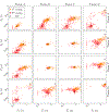
Scatter plots showing the estimated T₁ and T₂ values in the multicompartment model for voxels containing tissue A and C. Different number of radial k-spaces spokes are tested at a fixed SNR of 10³. The two clusters corresponding to the two tissues concentrate more tightly around the ground truth (GT, marked with black crosses) as the number of spokes increases.

Figure 21:

The normalized root-mean-square errors (NRMSE) in the T₁ and T₂ estimates are plotted as a function of the SNR when acquiring 8 radial k-space spokes. The NRMSE is defined as the root-mean square of the ∆T₁,₂/T₁,₂. The results are averaged over 10 realizations of the noise, and the hardly-visible error bars depict one standard deviation of the variation between different noise realizations. The NRMSE was also computed excluding voxels containing a combination of tissue B and C, because the corresponding fingerprints are highly correlated.

Figure 22:

Scatter plots showing the estimated T₁ and T₂ values in the multicompartment model for voxels containing tissue A and C. The data was reconstructed from 16 radial k-space spokes. The two clusters corresponding to the two tissues concentrate more tightly around the ground truth (GT, marked with black crosses) as the SNR increases.

Figure 23:

Scatter plots showing the estimated T₁ and T₂ values in the multicompartment model for simulated data with an SNR = 100 and using 16 radial k-space spokes. The tissues contained in those voxels are indicated above and to the right. The ground truth value of their respective relaxation times is marked with black crosses.

Figure 24:

Computer-aided design (left) and the corresponding 3D-printed phantom (right) used for the phantom evaluation. It contains two layers, one with four horizontal and one with four vertical bars. Imaging a slice that contains both layers results in the same effective structure as the numerical phantom shown in Figure 14.

Figure 25:

The depicted parameter maps were reconstructed from data measured in a phantom and using a single-compartment model. The data were acquired using 8 radial k-space spokes. The colorbar is adjusted so that distinct colors correspond to the parameters of the gold-standard reference measurements: red, yellow green and blue represent the solutions A-D.

Figure 26:

The parameter maps of the scanned phantom was reconstructed using the proposed multicompartment method. The data were acquired using eight radial k-space spokes. The three compartments with the highest detected proton density are shown here, and are sorted in each voxel according to their 𝓁₂-norm distance to the origin in T₁-T₂ space. The colorbar is adjusted so that distinct colors correspond to the parameters of the gold-standard reference measurements: red, yellow green and blue represent the four solutions.

Figure 27:

The scatter plot shows the estimated relaxation times of the measured phantom at the example of voxels containing different combinations of compartments. For comparison, the estimates obtained from the single-compartment (SC) are shown, as well as the gold-standard (GS) values measured on the diagonal, where only a single compartment is present. The rectangles represent the standard deviation of the gold-standard measurement.

References

1. Allerhand A and Gutowsky HS. Spin-Echo NMR Studies of Chemical Exchange. I. Some General Aspects. The Journal of Chemical Physics, 41:2115–2126, Oct. 1964. - PubMed
1. Assländer J, Cloos MA, Knoll F, Sodickson DK, Hennig J, and Lattanzi R. Low rank alternating direction method of multipliers reconstruction for mr fingerprinting. Magnetic Resonance in Medicine, 79(1):83–96, 2018. - PMC - PubMed
1. Assländer J, Glaser SJ, and Hennig J. Pseudo steady-state free precession for mr-fingerprinting. Magnetic resonance in medicine, 77(3):1151–1161, 2017. - PubMed
1. Assländer J, Lattanzi R, Sodickson DK, and Cloos MA. Relaxation in Spherical Coordinates: Analysis and Optimization of pseudo-SSFP based MR-Fingerprinting. arXiv, 1703.00481(v1), 2017.
1. Beck A and Teboulle M. A fast iterative shrinkage-thresholding algorithm for linear inverse problems. SIAM journal on imaging sciences, 2(1):183–202, 2009.