The Proteogenomic Landscape of Curable Prostate Cancer

Abstract

DNA sequencing has identified recurrent mutations that drive the aggressiveness of prostate cancers. Surprisingly, the influence of genomic, epigenomic, and transcriptomic dysregulation on the tumor proteome remains poorly understood. We profiled the genomes, epigenomes, transcriptomes, and proteomes of 76 localized, intermediate-risk prostate cancers. We discovered that the genomic subtypes of prostate cancer converge on five proteomic subtypes, with distinct clinical trajectories. ETS fusions, the most common alteration in prostate tumors, affect different genes and pathways in the proteome and transcriptome. Globally, mRNA abundance changes explain only ∼10% of protein abundance variability. As a result, prognostic biomarkers combining genomic or epigenomic features with proteomic ones significantly outperform biomarkers comprised of a single data type.

Keywords: biomarker; epigenome; genome; multi-omic features; prostate cancer; proteome; transcriptome.

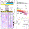
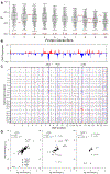
Figure 1.. Proteomic landscape of curable prostate cancer

(A) Study overview showing the clinical characteristics of the cohort (n = 76) and the number of samples with whole genome sequencing, RNA-Sequencing, methylation data and CHiP-Seq data. Mass spectrometry yielded 7,054 protein groups, whose abundance was corrected for batch effects, and missing values were imputed prior to downstream analyses. (B) Distribution of protein quantitation measured as median intensity by the number of samples they are detected in. Bar plot on top shows the total counts of proteins quantified in various number of samples. Missing values were omitted when calculating the median. (C) Consensus clustering of 76 patients (K=5) using the top 25% most variable genes (n=1,800, K=5). Clinical covariates are shown in the heatmap above, indicating for each patient; biochemical relapse (BCR), clinical ISUP grade (cISUP), PSA levels, clinical T category (cT), and age at treatment (years). (D) Subtypes identified from consensus clustering were evaluated to determine their association with BCR. A Cox PH model was fitted for subtype C2, C3, C4 and C5 against the baseline group of subtype C1. Hazard ratios and p values are shown with confidence intervals in parentheses. Abbreviations: International Society for Urological Pathology (ISUP), prostate specific antigen (PSA), hazard ratio (HR) See also Figure S1, Tables S1–S4, and Data S1.

Figure 2.. Transcriptomic and Proteomic Consequences of ETS fusions

(A) Comparison of the difference in protein and mRNA abundance observed between samples with an ETS gene fusion and those without. Analysis includes 55 samples with matched RNA-Seq and protein data in 255 genes as 22 genes were removed due to a high proportion of missing protein data. Color indicates which protein abundance decile the gene is in, where purple indicates the most abundant. (B) Number of overlapping ETS gene fusion associated genes between protein, mRNA, methylation, H3K27Ac, and copy number status. Barplot on the left indicates the total number of associated genes in that data type. Barplot on top shows number of genes in the singleton or intersection groups as indicated by the dots below. (C) Pathway enrichment analysis performed using g:Profiler on the five sets of genes associated with ETS gene fusions in the different data types. Large clusters of similar pathways are outlined in yellow and labeled. Singleton nodes were omitted. No pathway enrichment was detected in copy number changes associated with ETS gene fusions. See also Figure S2.

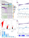
Figure 3.. Trans proteomic effects of somatic CNAs

(A) Distribution of RNA-protein Spearman’s ρ in each decile of protein abundance. Median correlations of each decile are indicated in red along the x-axis. Known genes of interest are highlighted and labeled in red. Boxplots depict the upper and lower quartiles, with the median shown as a solid line; whiskers indicate 1.5 times the interquartile range (IQR). Data points outside the IQR are shown. (B) The proportion of samples that contain copy number amplifications (red) and deletions (blue) in 210 samples with mRNA data. (C) The heatmap displays a global overview of the difference in mRNA abundance for each CNA locus comparing abundance from samples with a CNA to those without. Positive fold changes (i.e. higher abundance in samples with an amplification) are shown in red, negative fold changes (i.e. lower abundance in samples with a deletion) are shown in blue (FDR < 0.05). The x-axis plots 23,068 CNAs and the y-axis plots 6,636 mRNA genes. Genes are ordered by chromosome location on both axes. (D) The fold change in mRNA and protein abundances in 55 matched samples (RNA Seq) comparing abundances in samples with a deletion and those without for PTEN, CD68, and NKX3–1. Only genes that show significant fold changes at the mRNA (Mann-Whitney U test; p < 0.05) and protein level (Mann-Whitney U test; p < 0.05) are plotted. See also Figures S3–S4, and Table S5.

Figure 4.. Integrated clustering of multi-omics data

(A) Distribution of the normalized mutual information (MI) for each data-type pair. Boxplots depict the upper and lower quartiles, with the median shown as a solid line; whiskers indicate 1.5 times the interquartile range (IQR). Data points outside the IQR are shown. (B) Consensus clustering of normalized mutual information for each data-type pair. Biomolecules are indicated in the covariates along the top. Each row represents a gene (n = 6,484) comparison for which all data-types exist. Adjacent plots indicate if genes are known to be associated with the selected pathways. Normalized MI are plotted as z-scores for visualization purposes. (C) Correlation of normalized mutual information between our cohort and TCGA in genes with MI above 0.05. Red dots indicate genes that had normalized MI about 0.05 in both our dataset and TCGA. (D) Percent variance explained of protein abundance modeled using copy number status, methylation, and mRNA abundance for a select set of genes known to be associated with prostate cancer. (E and F) Integrated distribution plots of KLK3 (E) and PTEN (F) showing CN state and z-scored protein, mRNA, and methylation abundances for each of the 76 samples ordered by increasing protein abundance. Abbreviations: Cellular Response to Stress (CRS), Extracellular Exosomes (ExExo) See also Figure S4 and Table S6.

Figure 5.. Protein abundance robustly predicts patient survival

(A) Hazard ratios were calculated using a Cox model on patient groups determined using median-dichotomized protein and RNA abundances. Shading of dots indicates statistical significance with selected genes labeled in red. (B) Kaplan-Meier (KM) plot for PUS1 protein (solid lines) and mRNA (dashed lines). A Cox model was fit with patients stratified into high and low abundance of PUS1 protein (75 patients) and mRNA (209 patients). (C) KM plot showing 10-year biochemical recurrence-free survival of patient groups as dichotomized by high and low protein abundance of ACAD8. (D) KM plot for ACAD8 in 73 tissue microarrays. Three slides were evaluated per sample, and patients were grouped into ‘low’ protein abundance if at least two slides reported heterogeneous or faint staining. Significance of association was calculated using a log-rank test between high and low abundance patient groups. (E) Null distribution of predictive accuracy for different biomolecules obtained from 10 million replicates of 100 randomly selected genes. For each replicate, a value for the area under the receiver-operator curve (AUC) was calculated using classification results from four-fold cross-validation in random forest. See also Figure S5.

References

1. Aryee MJ, Jaffe AE, Corrada-Bravo H, Ladd-Acosta C, Feinberg AP, Hansen KD, and Irizarry RA (2014). Minfi: A flexible and comprehensive Bioconductor package for the analysis of Infinium DNA methylation microarrays. Bioinformatics 30, 1363–1369. - PMC - PubMed
1. Baca SC, Prandi D, Lawrence MS, Mosquera JM, Romanel A, Drier Y, Park K, Kitabayashi N, MacDonald TY, Ghandi M, et al. (2013). Punctuated evolution of prostate cancer genomes. Cell 153, 666–677. - PMC - PubMed
1. Bhandari V, Hoey C, Liu LY, Lalonde E, Ray J, Livingstone J, Lesurf R, Shiah Y-J, Vujcic T, Huang X, et al. (2019). Molecular landmarks of tumor hypoxia across cancer types. Nat. Genet doi:10.1038/s41588-018-0318-2 - DOI - PubMed
1. Blume-Jensen P, Berman DM, Rimm DL, Shipitsin M, Putzi M, Nifong TP, Small C, Choudhury S, Capela T, Coupal L, et al. (2015). Development and Clinical Validation of an In Situ Biopsy-Based Multimarker Assay for Risk Stratification in Prostate Cancer. Clin. Cancer Res. 21, 2591–2600. - PubMed
1. Bose R, Karthaus WR, Armenia J, Abida W, Iaquinta PJ, Zhang Z, Wongvipat J, Wasmuth EV, Shah N, Sullivan PS, et al. (2017). ERF mutations reveal a balance of ETS factors controlling prostate oncogenesis. Nature 546, 671–675. - PMC - PubMed
Publication types