Designing a rigorous microscopy experiment: Validating methods and avoiding bias

Abstract

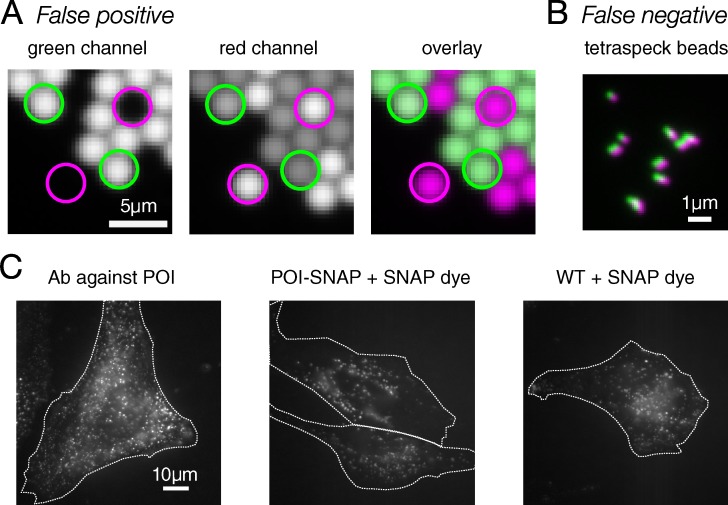
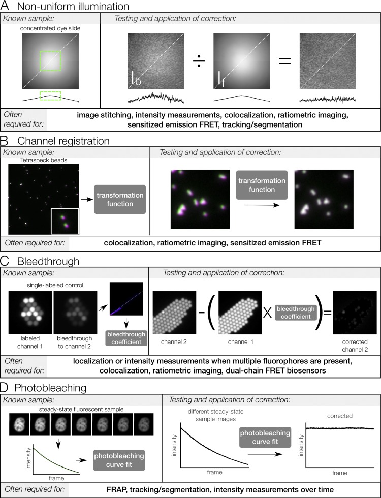
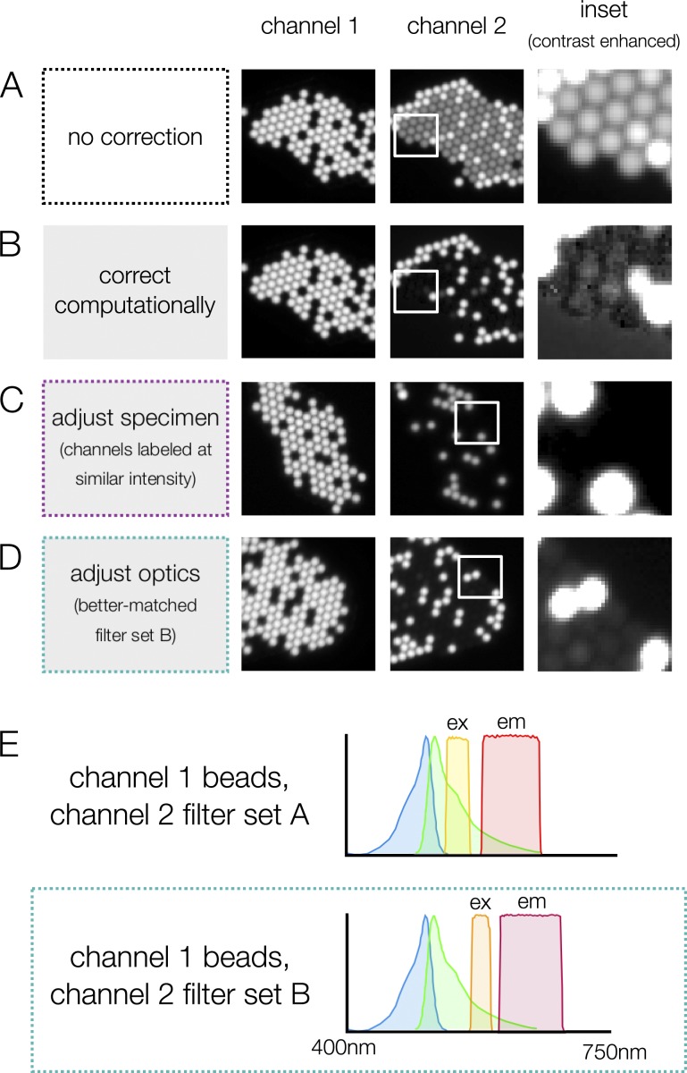
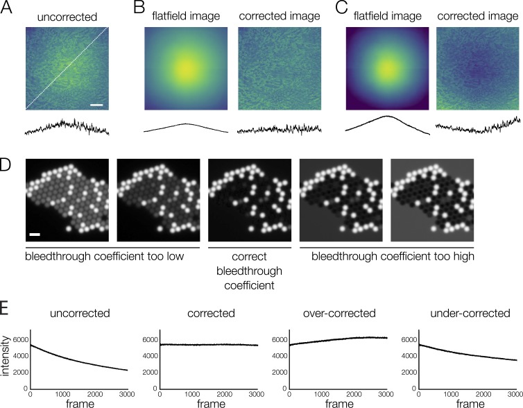
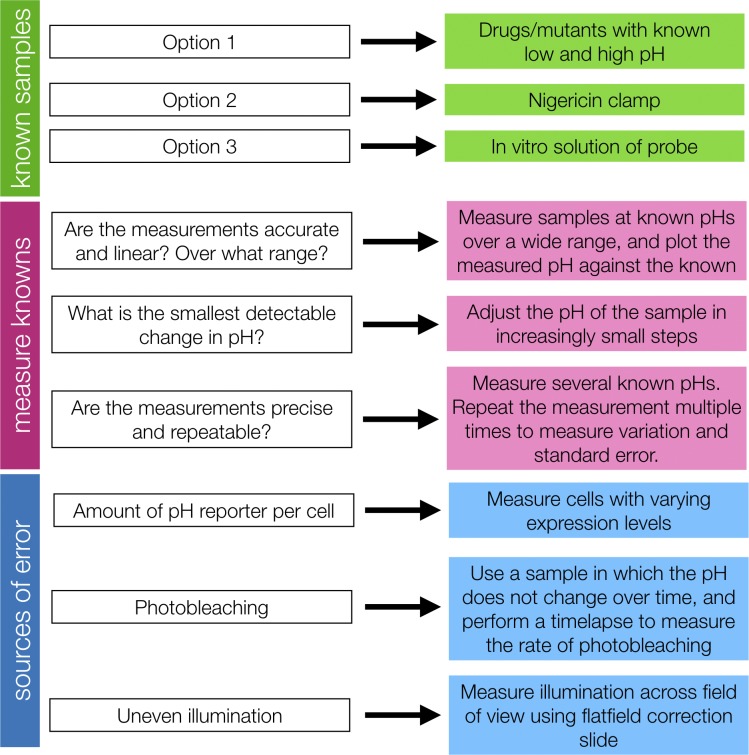
Images generated by a microscope are never a perfect representation of the biological specimen. Microscopes and specimen preparation methods are prone to error and can impart images with unintended attributes that might be misconstrued as belonging to the biological specimen. In addition, our brains are wired to quickly interpret what we see, and with an unconscious bias toward that which makes the most sense to us based on our current understanding. Unaddressed errors in microscopy images combined with the bias we bring to visual interpretation of images can lead to false conclusions and irreproducible imaging data. Here we review important aspects of designing a rigorous light microscopy experiment: validation of methods used to prepare samples and of imaging system performance, identification and correction of errors, and strategies for avoiding bias in the acquisition and analysis of images.

Figure 1.

Image errors can lead to incorrect results. (A) Bleed-through causes a false-positive colocalization result. Green and red beads were mixed and mounted together. There are no beads in these samples/images that are labeled with both green and red dye. With this filter and sample combination, there is significant bleed-through from the green beads into the red channel (see green circles). Pearson’s R for colocalization is 0.67. Since no pixel that contains green fluorophore also contains red fluorophore, there should be no correlation. (B) Channel misregistration causes a false-negative colocalization result. Tetraspeck beads are labeled with four dyes, including dyes imaged in the green and red channels here. Because each bead is labeled with both dyes, there should be complete colocalization between channels, with an expected Pearson’s R of 1. However, the imaging system has introduced significant misregistration between the channels, leading to a Pearson’s R of 0.66. (C) Nonspecific dye binding leads to a false-positive result. A significant level of nonspecific binding of SNAP dye to cells containing no SNAP tag (WT + SNAP dye) looks qualitatively similar to both cells containing a SNAP tag fused to the POI and immunofluorescence against POI. White dotted lines indicate cell outlines.

Figure 2.

Measurement and computational correction of image errors. Known samples are used to measure systematic errors in microscopy images. From the measurement, a correction can be generated, tested, and applied to experimental images. Correction procedures are summarized here and some steps (e.g., background subtraction) have been omitted. Please refer to the main text for references that cover these corrections in more detail. (A) Illumination nonuniformity. Concentrated dye is mounted between a coverslip and a slide and sealed. This dye, if sufficiently concentrated, acts as a thin, uniformly fluorescent sample (see Model and Burkhardt, 2001; Model, 2006). This “flat-field image” can be used to determine a region with minimal illumination variation (green box) or can be used to correct experimental images. The correction is tested by applying to a biological sample of roughly uniform intensity across the field of view, here a kidney section labeled with AlexaFluor568 phalloidin. Line scans below each image show intensity along the indicated white dotted line. (B) Channel registration. Tetraspeck beads are infused with four fluorescent dyes, including the green and red dyes imaged here (pseudo-colored green and magenta, respectively). Because the images of the beads in each channel should overlay perfectly, they can be used to generate a transformation matrix that describes the transformation needed to align the images. This matrix is then tested by using it to correct a different image of Tetraspeck beads. Once tested, the matrix can be used to register channels of experimental images. (C) Bleed-through. Samples labeled with a single fluorophore are used to measure bleed-through by imaging all channels with the same settings used for acquisition in the experiment. Here, 2.5-µm beads labeled with a dye corresponding to channel 1 are used. The intensity of bleed-through into channel 2 is plotted as a function of intensity of channel 1, and a linear regression of this plot is used to generate a bleed-through coefficient. This coefficient is then tested by applying to a different single-labeled control image and verifying that bleed-through into channel 2 is reduced. Once tested, the bleed-through coefficient can be used to correct for bleed-through in experimental images (provided channels are properly registered, as described above). (D) Photobleaching. Samples with steady-state fluorescence are used to generate a photobleaching curve under the planned experimental conditions. This curve is fit to an exponential function, which is then tested by correcting a different set of images of the steady-state sample. Once tested, the correction can be applied to experimental images under similar conditions; that is, if the correction is to be used across multiple days or sessions, it should be validated on images collected on multiple days. FRET, Förster resonance energy transfer.

Figure 3.

Image errors can be corrected in multiple ways. (A) Without correction, there is significant bleed-through from channel 1 into channel 2 (dimmer spots in channel 2 image). (B) Bleed-through can be corrected computationally (Fig. 2 C), but the correction can lead to artifacts that skew intensity measurements (see contrast-enhanced inset). Bleed-through can also be reduced by adjusting the specimen (C) or adjusting optics (D) in the microscope. Whether or not bleed-through is a problem for a particular experiment depends on the relative intensity of the fluorophores. In A, the beads in channel 1 are >300× brighter than the beads in channel 2; in C, beads of similar intensity are used, and bleed-through is no longer detectable. In D, a spectrally shifted filter set (E) is used to reduce bleed-through. At a glance, neither of these filter sets appears to have significant overlap with the excitation spectrum of the dye, but the small amount of overlap is exacerbated by the large difference in intensity between the channels.

Figure 4.

Image corrections must be tested carefully. (A–C) Flatfield correction. (B) When the flatfield image truly represents the illumination distribution, the uniformity of the test image (kidney section labeled with AlexaFluor568 WGA) is improved (see line scans below images, measured at the location indicated by the dotted white line in A). (C) When the correction is performed with a flatfield image that does not represent the illumination distribution, or has been normalized incorrectly, the test image is less uniform after correction. Correcting with an inaccurate flatfield image can add error to quantitative intensity measurements. If the flatfield image does not perform well in tests, a better solution is to define a subregion with less variable intensity (see Fig. 2 A). (D) Bleed-through correction. If the estimated bleed-through coefficient is inaccurate, bleed-through correction can lead to artifacts in the image that will add error to quantitative intensity measurements. Because these images contain no overlap between channels (mixed beads as in previous bleed-through figures, channel 2 shown), incorrect bleed-through coefficients show obvious artifacts; artifacts will be less obvious in experimental images with some overlap in signal. The bleed-through coefficient should be tested on single-labeled sample images before applying to experimental images. (E) Photobleaching correction. The sample in this example is fixed, meaning variation in intensity is due only to photobleaching and detector noise. If the rate of photobleaching is correctly measured, the corrected intensity values remain constant over time. If the rate of photobleaching is over- or underestimated, the corrected intensity values are no longer constant. Inaccurate corrections are obvious when applied to a steady-state sample, but over- or undercorrection may be impossible to detect when applied to a signal that varies over time. Scale bars: (A) 100 μm, (D) 5 μm.

Figure 5.

Measurement validation example: using a fluorescent biosensor to measure subcellular pH. To validate measurements, known samples (green) are required. These knowns can be used to characterize the dynamic range, linearity, and repeatability of measurements (magenta) and sources of error in the measurements (blue). For more information about pH measurements, see Grillo-Hill et al. (2014) and O’Connor and Silver (2013).

Figure 6.

Visual inspection of images is prone to confirmation bias. (A and B) In this example, cells labeled with a fluorescent nuclear marker exist in two populations, one with very bright nuclear labeling and the other with much dimmer labeling. If the image is autoscaled (A), the dimmer population is invisible, but brightness and contrast adjustments show that there is also a population of cells with lower intensity labeling (B). Making conclusions based on images displayed using autoscale (the most common default display in image acquisition programs), rather than measuring image intensity values, could lead to inaccurate conclusions. A researcher who is convinced by the image display because it represents the expected result, and therefore makes the decision not to complete a full quantitative analysis, is subject to confirmation bias. Scale bar: 50 μm. (C) Measured intensity of the nuclei in the images. Each dot represents the mean intensity of one nucleus.

References

1. Allan V.J., editor. 2000. Protein localization by fluorescent microscopy : a practical approach. Oxford University Press, Oxford.
1. Allan C., Burel J.M., Moore J., Blackburn C., Linkert M., Loynton S., Macdonald D., Moore W.J., Neves C., Patterson A., et al. . 2012. OMERO: flexible, model-driven data management for experimental biology. Nat. Methods. 9:245–253. 10.1038/nmeth.1896 - DOI - PMC - PubMed
1. Allison D.G., and Sattenstall M.A.. 2007. The influence of green fluorescent protein incorporation on bacterial physiology: a note of caution. J. Appl. Microbiol. 103:318–324. 10.1111/j.1365-2672.2006.03243.x - DOI - PubMed
1. Arganda-Carreras I., Kaynig V., Rueden C., Eliceiri K.W., Schindelin J., Cardona A., and Sebastian Seung H.. 2017. Trainable Weka Segmentation: a machine learning tool for microscopy pixel classification. Bioinformatics. 33:2424–2426. 10.1093/bioinformatics/btx180 - DOI - PubMed
1. Aubin J.E. 1979. Autofluorescence of viable cultured mammalian cells. J. Histochem. Cytochem. 27:36–43. 10.1177/27.1.220325 - DOI - PubMed