Gene-Environment Interaction in the Era of Precision Medicine

Abstract

Innovative analytical frameworks are required to capture the complex gene-environment interactions. We investigate the insufficiency of commonly used models for disease genome analysis and suggest considering genetic interactions in complex diseases. For non-genetic factors, we study the emerging wearable technologies that have enabled quantification of physiological and environmental factors at an unprecedented breadth and depth. We propose a Bayesian framework to hierarchically model personalized gene-environmental interaction to enable precision health and medicine.

Figure 1.. Frameworks for Disease Genome Analysis

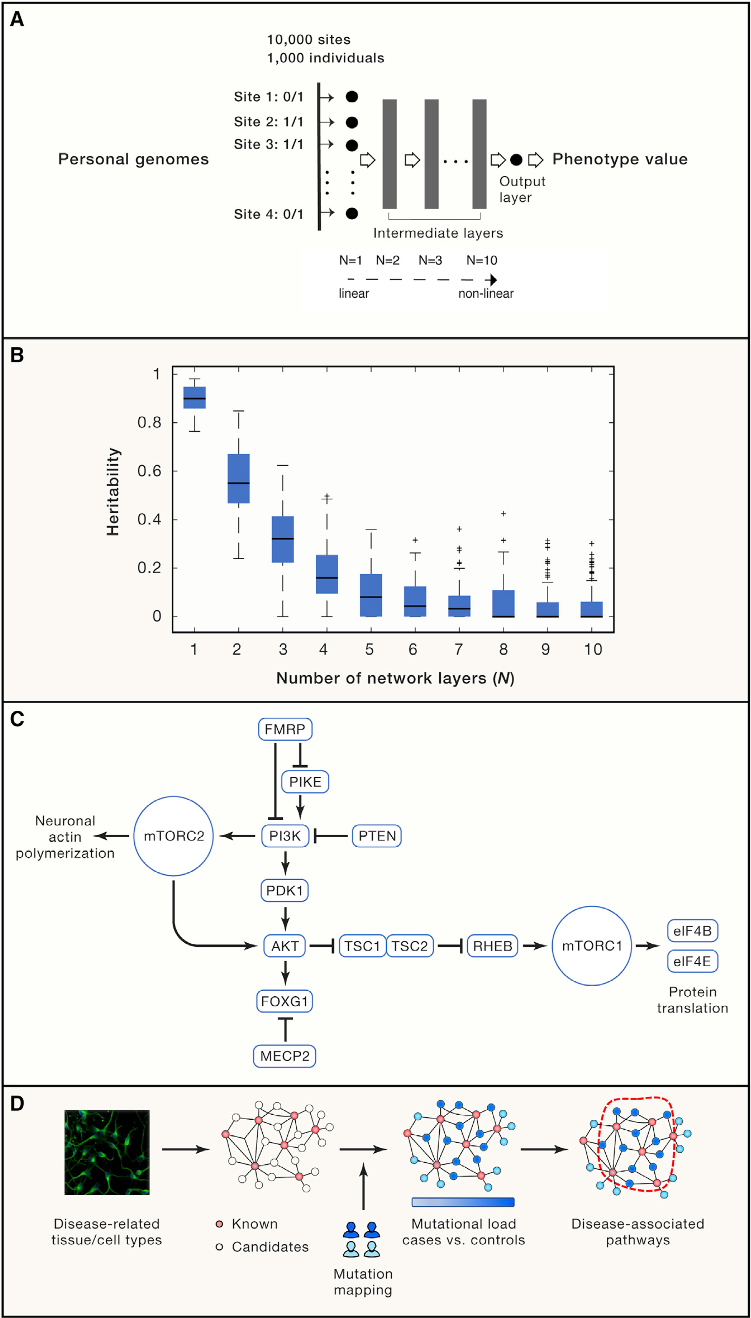
(A) A simulation study for identifying the potential source of missing heritability employing a deep neural network. 10,000 polymorphic sites from 1,000 individuals were randomly extracted from a published GWAS (Hong et al., 2017), which were then fed into a pre-configured (with a fixed weight on each edge) deep neural network with varying layers (from N = 1 to N = 10) to model the genotype-phenotype mapping. In particular, N = 1 is a linear regression model taking genotype input across all polymorphic sites (only the input layer and no intermediate layer), and their linear combination generates the output of a phenotype value, thereby representing the conventional additive genetic model. When multiple intermediate layers are involved (N > 1), the aggregated signal will be non-linearly transformed multiple times, as such N = 10 is a deep neural network representing a highly non-linear mapping from genotypes to a phenotypic trait. The network output is the phenotype value for each person that is deterministically derived from one’s genotypes after deep neural network transformation. We configured 5,000 nodes in each intermediate layer with a Sigmoid transfer function. For each N, the simulation was replicated for 100 times by setting network weights based on a standard normal distribution. Details about the simulation experiment. We input the genotypes of each individual into a feedforward neural network defined as: f₁ = σ(W₁x + b₁)(i) f₂ = σ(W₂f₁ + b₂)(ii) ... f_i = σ(W_if_i−1 + b_i)(iii) ... f_N−1 = σ(W_N−1f_N−2 + b_N−1)(iv) y = W_Nf_N−1 + b_N(v) Where N>1 in Equations (i-v), and f_i is the output from the i-th layer of the network. When N=1, the above equations degenerate to y = W₁x + b. Note that x∈R¹⁰⁰⁰⁰ is the genotype vector; σ is the sigmoid function; W_i and b_i (i = 1, …, N) are the weight matrix and bias term for each layer, respectively. Specifically, we defined W₁∈R^5000×10000 for the input layer, W_N∈R^1×5000 for the output layer and W_i∈R^5000×5000 for the intermediate layers. In the simulation experiment, we varied the number of layers from N = 1 to N = 10 to incrementally increase model complexity, i.e., the degree of non-linearity. For each N, we replicated the simulation 100 times. For each time, we kept the network structure unchanged and only configured a new set of weights and the bias term by sampling from a standard normal distribution independently, i.e., $\mathcal{N}(0,1)$. (B) The missed heritability is proportional to systems complexity using the commonly used linear mixture model (implemented by the GCTA toolkit). (C) An example of the PI3K/AKT/mTOR pathway, where most its member proteins are associated with neurodevelopmental diseases. (D) A systems biology strategy using multi-omics data to identify pathways significantly affected by disease-associated pathways. Biological pathways are first constructed using multi-omics profiling techniques in disease-related tissue/cell types, seeded with known disease-associated genes. Genomic mutations were then mapped onto the experimentally derived network to identify a compact sub-network most enriched for patient-specific mutations, which reveals disease-associated pathways.

Figure 2.. Wearable Sensors for Health Management and Physiological Data Acquisition

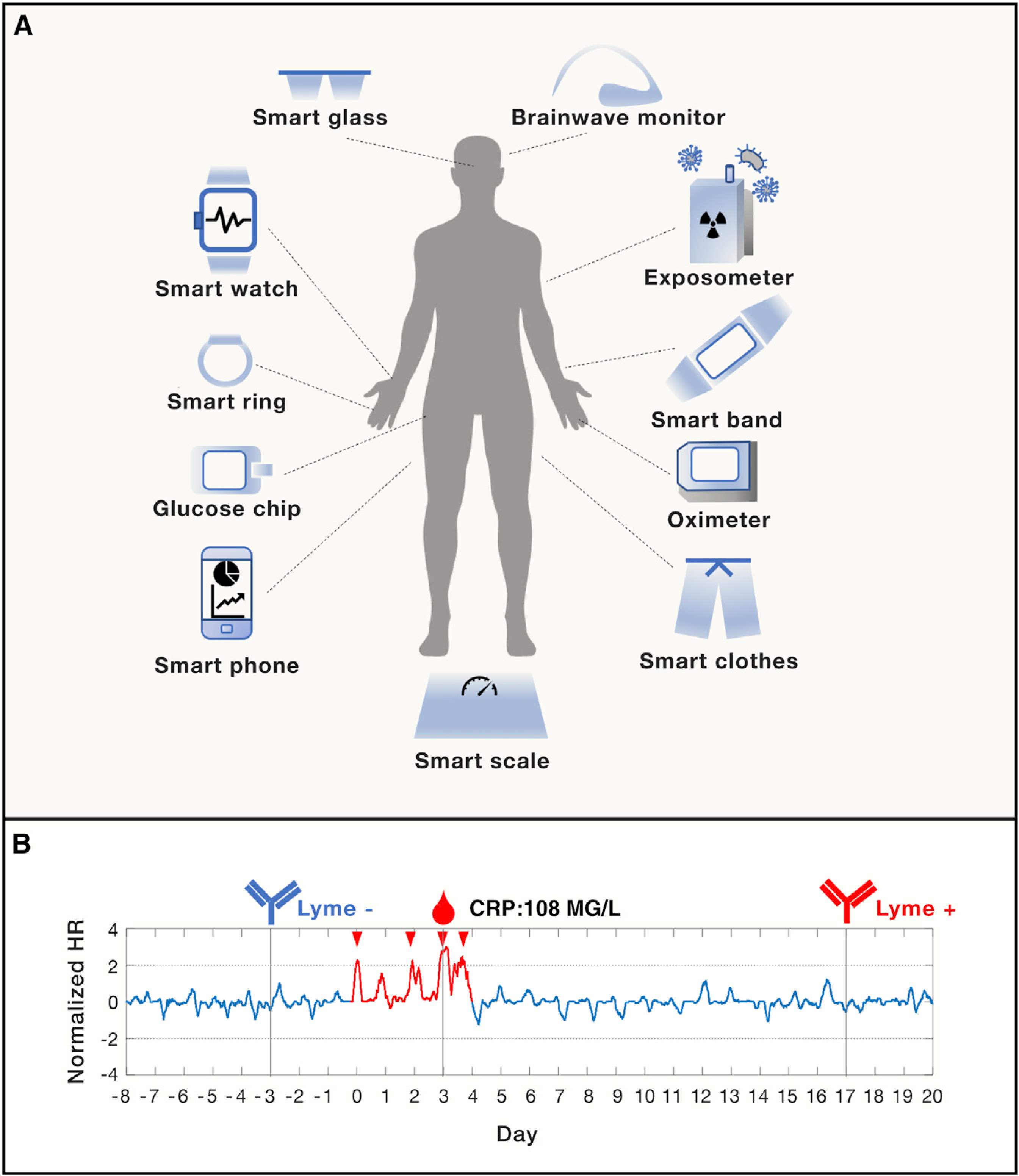
(A) An overview of existing wearable sensors acquiring human physiological and environmental data in real time. (B) Early detection of Lyme disease using smart watch. The normalized heart rate (HR) peaked during the Lyme infection event (in red) with a CRP (c-reactive protein) value of 108 MG/L (day 0 to day 4). The infection was confirmed by negative and positive Lyme antibody testing before (day −3) and after the infection event (day 17, when the formal diagnosis was made).

Figure 3.. A Bayesian View of Gene-Environment Interaction

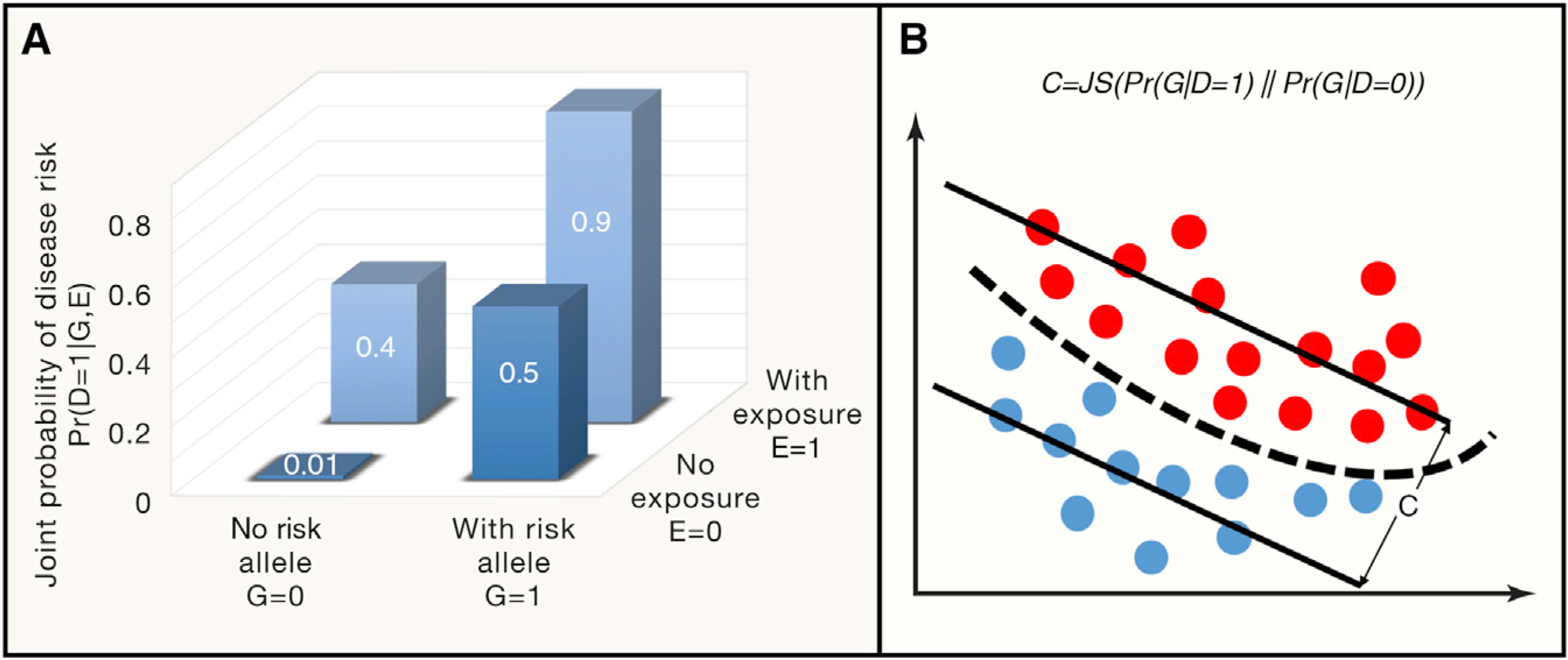
(A) A simplified example of BADGE illustrates the conditional dependency between genetic and environmental factors that determine the joint probability of disease outcome. According to Equations 1, 2, 3, 4, and 5 in the main text, assuming the risk allele frequency is Pr(G = 1) = 0.15 and the chance to be exposed to the environmental toxicant is Pr(E = 1) = 0.24, with some statistical inference procedures, one can readily determine disease prevalence Pr(D = 1) = 0.18, disease risk with and without environmental exposure at Pr(D = 1|E = 1) = 0.48 and Pr(D = 1|E = 0) = 0.08, respectively. Averaging out environmental factors, risk from personal genomes can be determined by Pr(D = 1|G = 1) = 0.60 and Pr(D = 1|G = 0) = 0.10, respectively, for individuals carrying or not carrying risk alleles. In the same vein, the genetic coefficient for this disease is 0.79 as defined in Equation 5. (B) Graphical representation of the genetic coefficient for a given disease, which is defined by the distributional difference of between the case (red dots) and control genomes (blue dots), quantified by Jensen–Shannon (JS) divergence.