Accuracy and precision of the RABBIT technique

Abstract

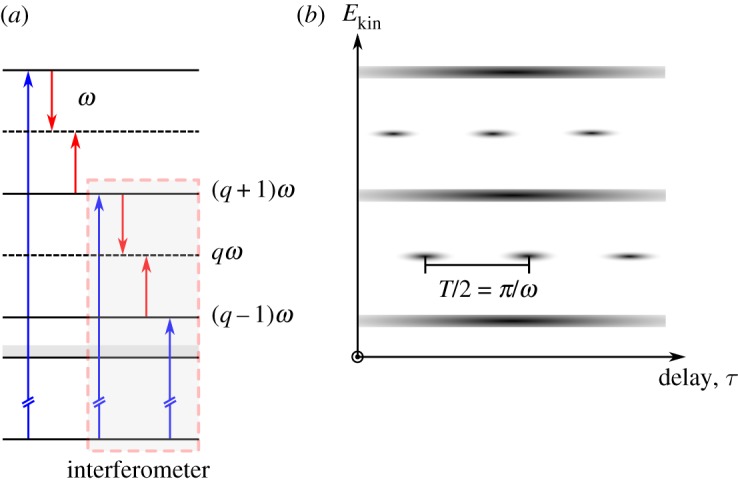
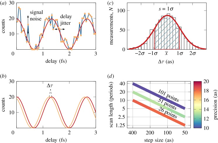
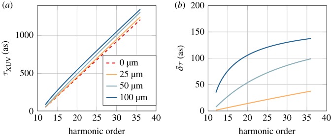
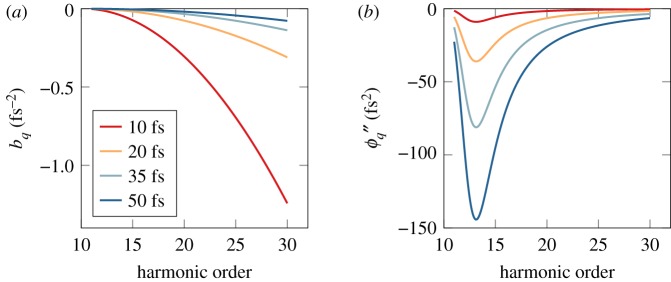
One of the most ubiquitous techniques within attosecond science is the so-called reconstruction of attosecond beating by interference of two-photon transitions (RABBIT). Originally proposed for the characterization of attosecond pulses, it has been successfully applied to the accurate determination of time delays in photoemission. Here, we examine in detail, using numerical simulations, the effect of the spatial and temporal properties of the light fields and of the experimental procedure on the accuracy of the method. This allows us to identify the necessary conditions to achieve the best temporal precision in RABBIT measurements. This article is part of the theme issue 'Measurement of ultrafast electronic and structural dynamics with X-rays'.

Keywords: RABBIT; attosecond physics; high-order harmonic generation; photoionization timedelays.

Figure 1.

Principle of RABBIT. Each sideband q makes up a quantum interferometer, one arm being the absorption of harmonic q − 1 followed by absorption of an IR photon, and the other the absorption of harmonic q + 1 followed by emission of an IR photon, leading to the same final energy. The intensity of the sideband oscillates as a function of the delay between the pulses, with an oscillation period of T/2, where T is the period of the fundamental, and the phase of this oscillation reveals information about the target system. (Online version in colour.)

Figure 2.

Illustration of the model used to simulate RABBIT traces. (a) A RABBIT oscillation, on which temporal jitter and signal fluctuations are added; (b) determination of the phase difference between the best fit and the original function; (c) after repetition of this procedure N times, the precision can be determined as the standard deviation of the distribution function; (d) precision (in colour) as a function of scan length and step size for different number of sampling points, with a temporal jitter, σ_t, of 25 as. No signal and background noise was taken into account.

Figure 3.

Effect of the spatial variation of the light fields. (a) ‘Measured’ group delay obtained by a RABBIT measurement integrated over the focal plane for different XUV beam waists as a function of the sideband order. (b) Difference δτ between the ‘measured’ group delay and the group delay at r = 0 for different XUV beam waists as a function of sideband order.

Figure 4.

Intrinsic femtosecond chirp of the XUV radiation. Chirp rate (a) and group delay dispersion (b) of individual harmonic for different pulse durations of the fundamental laser.

Figure 5.

Effect of the chirp rate as a function of the fundamental pulse duration in RABBIT measurement. (a,b) Simulated scans in helium are exhibited for pulses of 5 fs and 30 fs, respectively. (c) The error in the phase retrieval for sideband 19 (at 5–6 eV kinetic energy). To ensure the convergence of the results, simulations were performed by varying the number of sampling points.

Figure 6.

Intra-sideband delay variation. (a) Numerical decomposition of harmonic 15. The dashed black curve is the amplitude of the pulse and the dashed grey curve is the phase. The pulse is decomposed into 13 different subpulses, each with a different constant phase. The blue curve shows the resulting amplitude and the red curve the resulting phase. (b) Delay variation in sideband 16 for different values of Δϕ_q′′. There is no blueshift. (c) Delay variation in sideband 32 for different blueshifts. The femtochirp of both harmonics is the same (−50 fs²). Note that in this case, the different phases do not span the same energy, as sidebands are broadened by the blueshift. In (b, c), the harmonic bandwidth is set to 150 meV and the probe bandwidth to 70 nm. The energy range is limited by a threshold of 30% of the maximum sideband intensity, below which we consider that the phase cannot be reliably extracted [43].

Figure 7.

RABBIT precision extracted from different sets of 1000 Monte Carlo simulations. (a) The temporal jitter was set to the four values indicated and the precision was calculated while the step size was decreased. (b) The temporal jitter was set to the four values indicated, and the step size was set to two times the magnitude of the jitter. The precision was calculated while the number of periods was increased. One period in this case was set to 1.33 fs (i.e. 800 nm wavelength).

Figure 8.

RABITT precision extracted from different sets of 1000 Monte Carlo simulations. (a) The maximum sideband amplitude was varied between 2 and 4086, and the Poisson noise was added to simulate the uncertainty of counting electrons in each delay step of the spectrogram. The simulations were repeated for a sample count of 60, 200 and 600 samples with a step size smaller than the Nyquist threshold for 2ω. (b) Precision as a function of relative background noise. The maximum sideband amplitude was set to 500 counts and the noise level was varied between 100% and 2% for the same three cases of sampling points.

Figure 9.

RABBIT precision as a function of number of sampling points and maximum allowed sideband oscillation measured in counts. Each diagonal line represents a line of constant acquisition time in a real experiment. The simulations were run with a jitter of 50 as, including statistical noise and a background level of 10%.

References

1. Krausz F, Ivanov M. 2009. Attosecond physics. Rev. Mod. Phys. 81, 163–234. (10.1103/RevModPhys.81.163) - DOI
1. Sansone G. et al. 2006. Isolated single-cycle attosecond pulses. Science 314, 443–446. (10.1126/science.1132838) - DOI - PubMed
1. Goulielmakis E. et al. 2008. Single-cycle nonlinear optics. Science 320, 1614–1617. (10.1126/science.1157846) - DOI - PubMed
1. Li J. et al. 2017. 53-attosecond X-ray pulses reach the carbon K-edge. Nat. Commun. 8, 186 (10.1038/s41467-017-00321-0) - DOI - PMC - PubMed
1. Gaumnitz T, Jain A, Pertot Y, Huppert M, Jordan I, Ardana-Lamas F, Worner HJ. 2017. Streaking of 43-attosecond soft-X-ray pulses generated by a passively CEP-stable mid-infrared driver. Opt. Express 25, 27 506–27 518. (10.1364/OE.25.027506) - DOI - PubMed