Network inference performance complexity: a consequence of topological, experimental and algorithmic determinants

Abstract

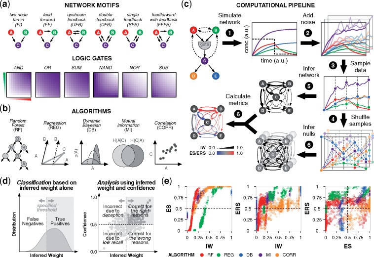
Motivation: Network inference algorithms aim to uncover key regulatory interactions governing cellular decision-making, disease progression and therapeutic interventions. Having an accurate blueprint of this regulation is essential for understanding and controlling cell behavior. However, the utility and impact of these approaches are limited because the ways in which various factors shape inference outcomes remain largely unknown.

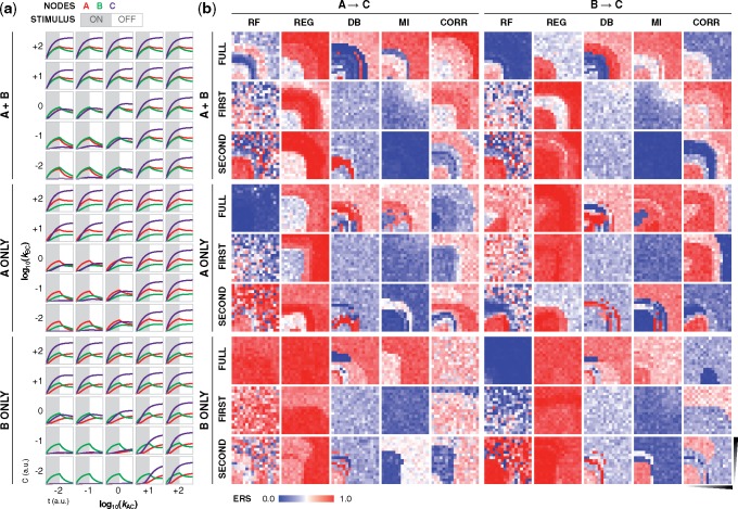
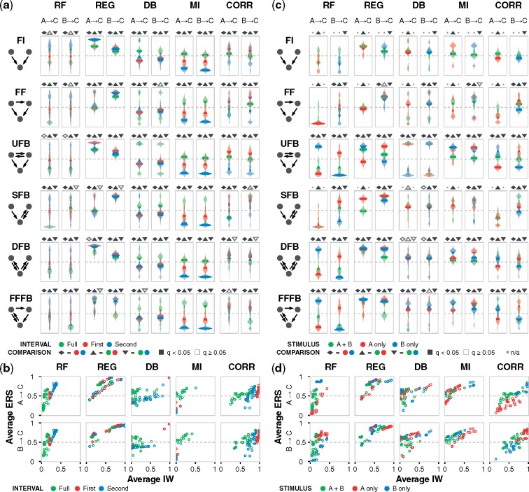
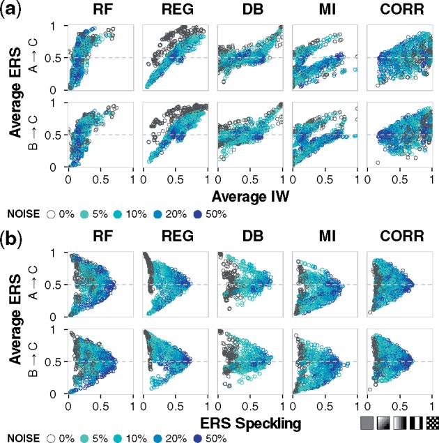
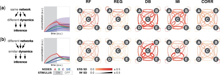
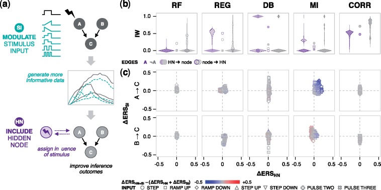
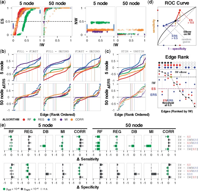
Results: We identify and systematically evaluate determinants of performance-including network properties, experimental design choices and data processing-by developing new metrics that quantify confidence across algorithms in comparable terms. We conducted a multifactorial analysis that demonstrates how stimulus target, regulatory kinetics, induction and resolution dynamics, and noise differentially impact widely used algorithms in significant and previously unrecognized ways. The results show how even if high-quality data are paired with high-performing algorithms, inferred models are sometimes susceptible to giving misleading conclusions. Lastly, we validate these findings and the utility of the confidence metrics using realistic in silico gene regulatory networks. This new characterization approach provides a way to more rigorously interpret how algorithms infer regulation from biological datasets.

Availability and implementation: Code is available at http://github.com/bagherilab/networkinference/.

Supplementary information: Supplementary data are available at Bioinformatics online.

Fig. 1.

Evaluating performance of network inference. (a) Networks differ in features such as motifs and gates. Gates differentially regulate node C based on the activity of nodes A and B. Color-coding (white to purple for low to high activity) characterizes node C in the fan-in motif. (b) Panel of algorithms that use distinct statistical learning methods. (c) Networks were simulated under different conditions to produce timecourse data. Noise was added before data samples were obtained, and true data were permuted to produce null data. Regulation was inferred by each algorithm, and inferred weights (IW) and null weights (NW) were compared to determine the confidence metrics ES and ERS. (d) Left: for a true edge, the two possible outcomes from a binary classification are true positive and false negative. The IW classification threshold depends on algorithm and context. Right: four-quadrant analysis of confidence and IW suggests reasons for algorithm performance. Confidence values above 0.5 indicate that a predicted model tends to outperform null models. Ideal outcomes are in the upper-right quadrant. (e) Left and middle: analysis with IW and confidence; right: comparison of confidence metrics. Results are color-coded by algorithm. For the 36 gate-motif combinations, inference outcomes are shown that are specific to edge A →C, using: nine representative kinetic parameters ($k_{\text{A}},k_{\text{B}}\in \{{10}^{-2}\hspace{0.17em}{10}^0\hspace{0.17em}{10}^2\}$), stimulus to nodes A and B, no added noise, and data sampled from the full timecourse

Fig. 2.

Network confidence varies across algorithms. (a) Trajectories of nodes A, B, and C, and (b) ERS for the two gate edges (A →C and B →C) for a network containing an FFFB motif and OR gate. ERS is provided as a function of stimulus condition (A only, B only or both A and B), time interval of input data (first half, second half and full timecourse), and gate kinetics (plot axes are in log space). Simulations in (a) show a subset of the kinetic landscape, and heatmaps in (b) show the full 17 × 17 landscape. Gate kinetics (a network property), stimulus target (an experimental choice), and time interval and algorithm (post-experimental choices) strongly affect inference outcomes. Additional simulation conditions and plots are in the Supplementary Material and online data browser

Fig. 3.

Performance depends on the sampled time interval and the stimulus target. (a) ERS distribution across the kinetic landscape for each algorithm, motif, and gate edge, with data for an OR gate and stimulus to nodes A and B. Violin plots for each landscape are color coded to reflect data sampled from the first half, second half, and full timecourse. Dashed lines indicate a confidence value of 0.5. Pairwise hypothesis testing for time intervals was performed using two-tailed Welch’s t-test, followed by multiple hypothesis correction using the Benjamini–Hochberg procedure for all tests within a given algorithm-edge group to obtain q values, as described in Materials and methods. Pairwise tests are indicated by the shapes above each subplot with statistically significant ($q<0.05$) outcomes filled-in. (b) Joint distribution of average IW and average ERS across the same landscape of motif-gate combinations and algorithm-edge groups. (c) ERS distribution for each algorithm, motif and gate edge, with data for an OR gate and data sampled from the full timecourse. Plots are color-coded based on node A, B, or both as the stimulus target(s). Absent violins are due to special cases that cannot be inferred (as algorithms do not interpret flat trajectories), and nonapplicable tests are denoted by a dot in place of a shape above subplots. (d) Joint distribution of average IW and average ERS. Additional simulation conditions and plots are in the Supplementary Material and online data browser

Fig. 4.

Robustness to noise in the sampled data. (a) Gaussian noise at 5, 10, 20 or 50% of the unit-scaled standard normal distribution was added to the sampled data. Joint distribution of average IW and average ERS. Each point summarizes results for a specific combination of motif, gate, stimulus target, and sampled time interval. (b) Joint distribution of ERS speckling and average ERS. With increasing levels of noise, the ERS speckling as a function of the kinetic landscape (Fig. 2b) increases and average algorithm performance converges to the null case. In the lower right, cartoon patterns depict an example trend for increased speckling. Additional simulation conditions and plots are available in the Supplementary Material and online data browser

Fig. 5.

Robustness to kinetic and topological variation. (a) A network topology can produce highly distinct data depending on the kinetic parameters. In the case shown, nine networks each have a FFFB motif, an AND gate, and stimulus to node A, but differ in gate kinetics. Left: the timecourse mean trajectories (line) and standard deviation (SD; shaded region) from the nine networks. Right: SD of IW (line width) and ERS (color coded) for each edge. Dashed lines indicate zero SD for IW. (b) In the reciprocal case, nine networks differ in motifs, gates, and kinetics, but all produce highly similar data. Individual plots are in the Supplementary Material, and additional simulation conditions are available in the online data browser

Fig. 6.

Modifications to the stimulus input and inclusion of stimulus data. (a) Depiction of the two strategies for improving algorithm performance: (i) new time-varying profiles for the stimulus input (SI), and (ii) providing stimulus information to algorithms through a new hidden node (HN). The SI panel includes ramp up, ramp down, two steps up, two steps down, two pulses, and three pulses. (b) For the HN strategy, violin plots show the IW distribution for inferred edges that are directed from the HN (shaded) or to the HN (striped), in relation to node A (purple), and nodes other than A ($\neg$A, gray). Circles between the pairs of violins indicate the mean of each violin. Each violin comprises IW distributions from 20 kinetic landscapes (FF and FFFB motifs, OR and AND gates, five noise levels). (c) Individual and combined effects of the two strategies. The signed change in ERS from implementing each modification individually is indicated by the axis values. Symbols denote the SI. Combined effects are color coded as synergistic (red), antagonistic (blue), or additive (gray). (Color version of this figure is available at Bioinformatics online.)

Fig. 7.

Validation using GeneNetWeaver networks. (a) IW–ES and IW–NW relationships for the original 5-node and validation 50-node networks, color-coded by algorithm. (b) Rank-ordered differences in ERS of two-parent fan-in edges between each pair of time intervals used as input data. Vertical lines indicate the x-coordinate where each trace changes sign. (c) Rank-ordered differences in ERS of two-parent fan-in edges when the parent node does or does not receive the stimulus. (d) Diagram depicting the principle of using different metrics to threshold edges in an inferred model. Upper: modulating the sensitivity-specificity trade-off without the constraint of remaining on the ROC curve. The larger arrows illustrate general trends using ES > 0.5 and IW$\cap$ERS > 0.5, but there are also other possible directions. Movement for the former depends on the initial location of comparison on the ROC curve, and movement for the latter is in a direction of lower sensitivity and higher specificity. Lower: in standard thresholding, edges are rank-ordered (x-axis) by value (y-axis) of IW (black) and only edges above the elbow are retained. Alternatively, ES (red) or ERS (blue) can be used, in combination with each other or IW, to retain high-confidence edges. Above the plot, filled-in circles indicate edges selected based on IW > elbow threshold, ES > 0.5, and ERS > 0.5. (e) Average difference in sensitivity and specificity using IW versus other approaches (rows). Error bars indicate standard deviation. Statistical significance from a one-tailed Wilcoxon signed-rank test is color coded. For example, if thresholding by ES > 0.5 gives significantly greater specificity than elbow-thresholding IW, this outcome is depicted by a green bar to the left of the zero coordinate. (Color version of this figure is available at Bioinformatics online.)

References

1. Ackers G.A., et al. (1982) Quantitative model for gene regulation by λ phage repressor. Proc. Natl. Acad. Sci. USA, 79, 1129–1133. - PMC - PubMed
1. Aibar S., et al. (2017) SCENIC: single-cell regulatory network inference and clustering. Nat. Methods, 14, 1083–1086. - PMC - PubMed
1. Alexopoulos L.G., et al. (2010) Networks inferred from biochemical data reveal profound differences in toll-like receptor and inflammatory signaling between normal and transformed hepatocytes. Mol. Cell. Proteomics, 9, 1849–1865. - PMC - PubMed
1. Balázsi G., et al. (2011) Cellular decision making and biological noise: from microbes to mammals. Cell, 144, 910–925. - PMC - PubMed
1. Bansal M., et al. (2007) How to infer gene networks from expression profiles. Mol. Syst. Biol., 3, 78. - PMC - PubMed
Publication types