Review
. 2019 Sep;92(1101):20181016.
doi: 10.1259/bjr.20181016. Epub 2019 Jul 26.

Introduction to Quantitative Susceptibility Mapping and Susceptibility Weighted Imaging

Affiliations
Review

Introduction to Quantitative Susceptibility Mapping and Susceptibility Weighted Imaging

Pascal P R Ruetten et al. Br J Radiol. 2019 Sep.

Abstract

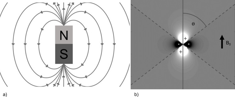
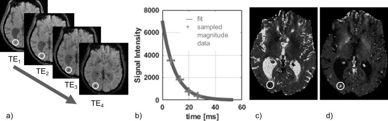
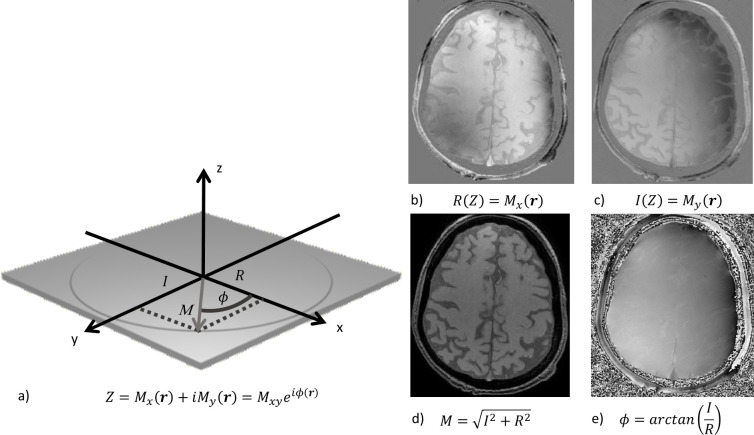
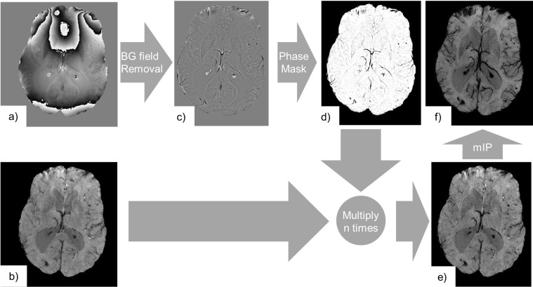
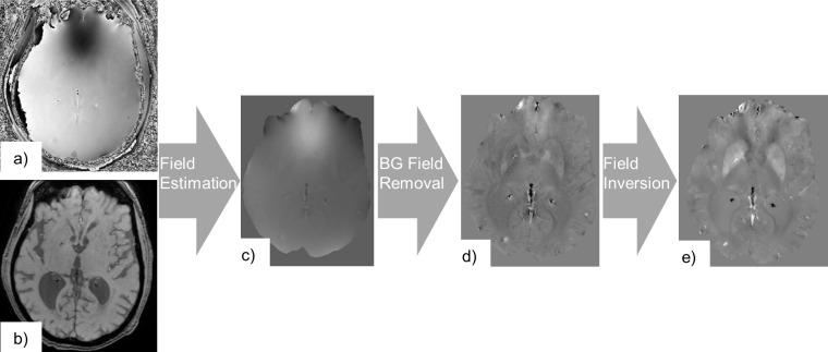
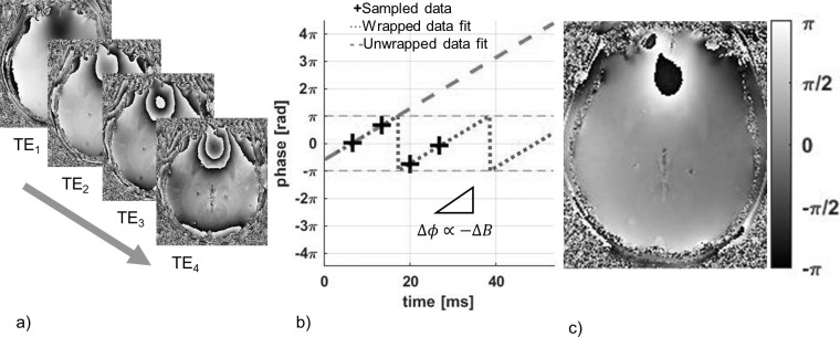
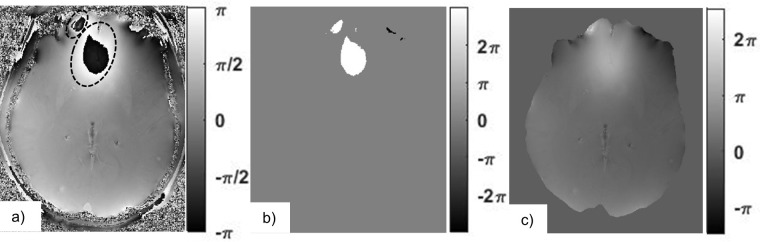
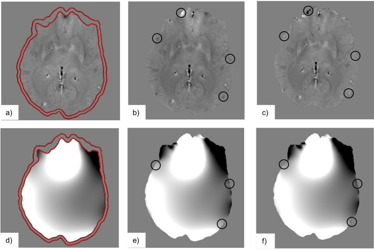
Quantitative Susceptibility Mapping (QSM) and Susceptibility Weighted Imaging (SWI) are MRI techniques that measure and display differences in the magnetization that is induced in tissues, i.e. their magnetic susceptibility, when placed in the strong external magnetic field of an MRI system. SWI produces images in which the contrast is heavily weighted by the intrinsic tissue magnetic susceptibility. It has been applied in a wide range of clinical applications. QSM is a further advancement of this technique that requires sophisticated post-processing in order to provide quantitative maps of tissue susceptibility. This review explains the steps involved in both SWI and QSM as well as describing some of their uses in both clinical and research applications.
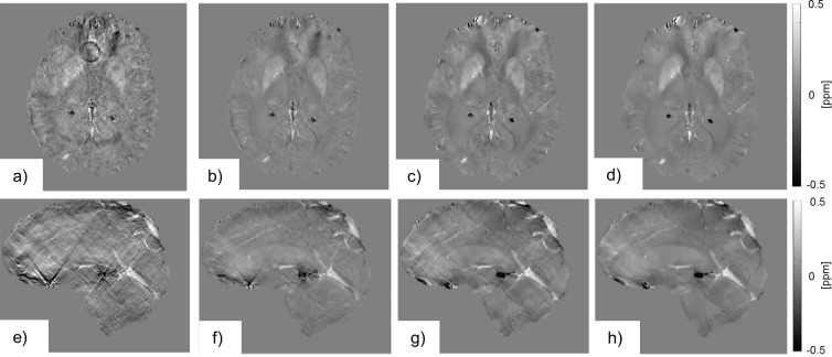
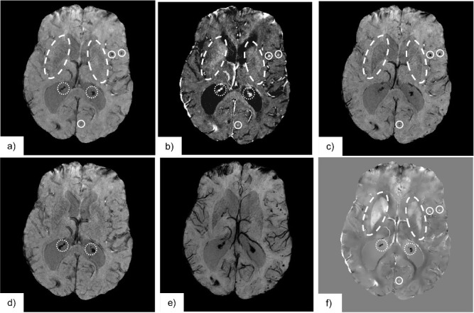

Figures

Figure 1.
Figure 1.
(a) Magnetic field lines of a magnetic dipole (b) Magnitude of the magnetic dipole field in the direction of ↑ B0. The values along the magic angle (Θ=54.7) are zero and there are lobes of positive and negative field strength, indicated as areas of relative hyper- and hypointensity respectively.
Figure 2.
Figure 2.
This figure illustrates T 2 */R 2 *-mapping: (a) Magnitude images of the brain acquired at four increasing echo times; the signal intensity in areas with a large susceptibility variation (in this example haemorrhage) decreases more rapidly than in the rest of the brain as indicated by the circle. (b) The time constant T 2 * is estimated by fitting an exponential decay to the magnitude signal intensity variation of every voxel over time; here we consider a sample from a high SNR ROI to illustrate the exponential shape of the signal decay. (c) The curve fitting results in a map of T 2 *, where the haemorrhage appears hypointense. (d) Sometimes a map of its reciprocal R 2 * is used instead, where the haemorrhage appears hyperintense. ROI,region of interest; SNR, signal-to-noise-ratio.
Figure 3.
Figure 3.
(a) The signal from the precessing proton spins which is acquired by the MR receiver is represented as a complex number with real (R) and imaginary (I) components from which a pixel-by-pixel signal magnitude and phase can be calculated. (b) Reconstruction of the real component of the magnetization. (c) Reconstruction of the imaginary component of the magnetization.(d) The calculated magnitude signal. (e)The calculated phase signal.
Figure 4.
Figure 4.
SWI consists of the processing of complex gradient echo MRI data, i.e. its phase (a) and magnitude components (b). Here, we used the fourth echo from a multi echo gradient echo acquisition (TE = 26.7 ms, TR = 32.0 ms, voxel size = 0.65×0.65×1.4 mm3). The phase (a) is high-pass filtered in order to remove the background phase (c). Contrast is generated by variations in the magnetic field generated by local susceptibility sources only. We can note that paramagnetic materials (haemorrhage, venous blood) appear as negative phase shifts, while diamagnetic materials (calcification) appear as positive phase shifts. The filtered phase data is further processed to generate a phase mask (d) that only darkens areas where the phase shift is negative. The magnitude image is subsequently multiplied n times (here n = 4) in order to generate the SWI (e). The phase mask was chosen to suppress signals from negative phase shifts only, so that the visibility of both haemorrhages and the venous vasculature was enhanced. A mIP may be employed to further emphasize paramagnetic venous vasculature across the stack of slices (f). mIP,minimum intensity projection; SWI, Susceptibility Weighted Imaging; TE, echo time; TR, repetition time.
Figure 5.
Figure 5.
QSM consists of the processing of complex gradient echo MRI data, i.e. its phase (a) and magnitude components (b). Here, we used a multiecho gradient echo acquisition (TE1 = 6.5 ms, echo spacing = 6.744 ms, #echoes = 4, TR = 32.0 ms, voxel size = 0.65×0.65×1.4 mm3). A map of field inhomogeneities ΔB is estimated from the phase data (c). Subsequently contributions from background fields are removed to extract a map of field inhomogeneities generated by susceptibility sources inside the ROI only, ΔBint (d). A dipole field inversion operation is performed on ΔBint to calculate the susceptibility map χ (e). ROI, region of interest; QSM, Quantitative Susceptibility Mapping; TE, echo time; TR, repetition time.
Figure 6.
Figure 6.
In order to estimate ΔB, the variation of the phase images (a) acquired from four increasing echo times (6.50, 13.24, 19.99, 26.73 ms) are monitored over time. By fitting a linear function to the multiecho phase data, phase wraps between subsequent echoes can be estimated and removed to estimate the slope of the phase variation over time and the corresponding value of ΔB (b). This is done for every voxel in the acquisition in order to generate a map of temporally unwrapped ΔB values scaled by a factor of γ2πΔTE (c).
Figure 7.
Figure 7.
The map of ΔB values scaled by a factor of γ2πΔTE (a) includes phase wraps that are outlined by dashed lines. Phase unwrapping algorithms identify these areas and add integer multiples of 2π (k2π) onto them. Here, bright areas indicate phase shifts of 2π, dark areas -2π and the rest is equal to zero (b). In the resulting unwrapped field map, all of the wrapping artifacts have been removed (c).
Figure 8.
Figure 8.
This figure shows the differences between the internally Bint (a–c) and externally generated field inhomogeneities Bext (d–f), as estimated by the algorithms SHARP (a, d), LBV (b, e), and PDF (c, f). Bext (d–f) is a large, slowly varying field component, that obscures the small local Bint (a–c). Due to different assumptions for the boundary conditions of the Background Field Removal algorithms we can see that there are some differences near the boundary indicated by the black circles on the LBV and PDF images. Furthermore, we can see that the field estimated by SHARP is reduced due to erosion (a, d). LBV, Laplacian boundary value; PDF,Projection onto Dipole Field; SHARP, Sophisticated Harmonic Artifact Reduction.
Figure 9.
Figure 9.
The figure shows the susceptibility maps generated by different dipole field inversion algorithms in axial (a–d) and sagittal (e–h) view. The susceptibility maps estimated using the TKD algorithm with a low threshold value (a, e) exhibits the characteristic streaking artifacts. By increasing the threshold value, we can see an improvement in image quality, but the contrast is reduced along with the streaking artifact (b, f). The MEDI algorithm is able to improve image quality even further, (c, g) and (d, h). By varying the regularization parameter, the susceptibility map gets smoother while the contrast is reduced (d, h). MEDI, Morphology Enabled Dipole Inversion; TKD, Truncated K-space Division.
Figure 10.
Figure 10.
The following demonstrates the application of the discussed susceptibility-based contrast to image anatomy and pathology in the brain: (a) T 2 *-weighted images indicate all susceptibility differences as hypointensities, such as calcifications (diamagnetic, χ§amp;lt;0, indicated by the dotted region), haemorrhages (paramagnetic, χ§amp;gt;0, indicated by the solid line region), iron rich structures (Putamen and Globus Pallidus, paramagnetic, χ§amp;gt;0, indicated by dashed line region) and deoxygenated blood in the venous vasculature (paramagnetic, χ§amp;gt;0) (b) R2 *-mapping, the reciprocal of the T 2 *-value, shows all the above as signal hyperintensities. (c) A susceptibility-weighted image employing a phase mask to reduce signal intensity for negative phase shifts only darkens areas of paramagnetic susceptibility. We have indicated the iron rich structures, haemorrhages, and veins. (d) A susceptibility-weighted image employing a phase mask to reduce signal intensity for positive phase shifts only emphasizes areas of diamagnetic susceptibility. We have indicated the calcifications by the dotted region. (e) A minimum intensity projection of the stack of susceptibility weighted images (c) improves visualization of the venous vasculature. (f) The susceptibility map is able to differentiate between regions where χ has negative and positive values, as areas of hypo- and hyperintensities, respectively.

References

    1. Haacke EM, Cheng NYC, House MJ, Liu Q, Neelavalli J, Ogg RJ, et al. . Imaging iron stores in the brain using magnetic resonance imaging. Magn Reson Imaging 2005; 23: 1–25. doi: 10.1016/j.mri.2004.10.001 - DOI - PubMed
    1. Schweser F, Deistung A, Lehr BW, Reichenbach JR. Differentiation between diamagnetic and paramagnetic cerebral lesions based on magnetic susceptibility mapping. Med Phys 2010; 37: 5165–78. doi: 10.1118/1.3481505 - DOI - PubMed
    1. Bonekamp D, Barker PB, Leigh R, van Zijl PCM, Li X. Susceptibility-based analysis of dynamic gadolinium bolus perfusion MRI. Magn Reson Med 2015; 73: 544–54. doi: 10.1002/mrm.25144 - DOI - PMC - PubMed
    1. Xu B, Spincemaille P, Liu T, Prince MR, Dutruel S, Gupta A, et al. . Quantification of cerebral perfusion using dynamic quantitative susceptibility mapping. Magn Reson Med 2015; 73: 1540–8. doi: 10.1002/mrm.25257 - DOI - PubMed
    1. Wong R, Chen X, Wang Y, Hu X, Jin MM. Visualizing and quantifying acute inflammation using ICAM-1 specific nanoparticles and MRI quantitative susceptibility mapping. Ann Biomed Eng 2012; 40: 1328–38. doi: 10.1007/s10439-011-0482-3 - DOI - PubMed

MeSH terms