Shallow Sparsely-Connected Autoencoders for Gene Set Projection

Abstract

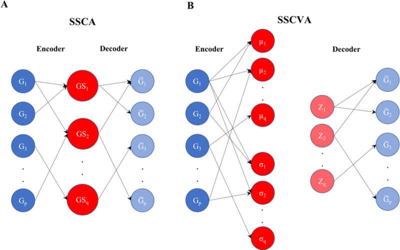
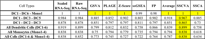
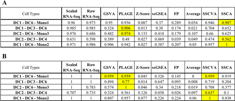
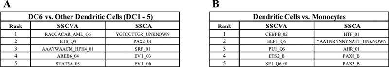
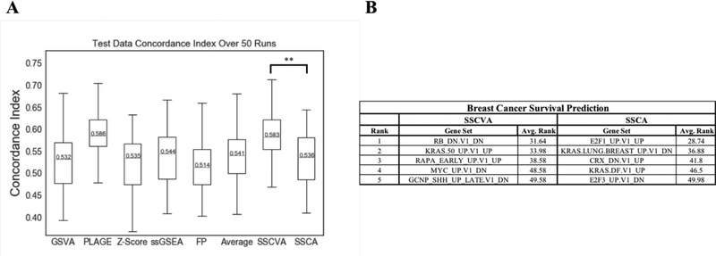
When analyzing biological data, it can be helpful to consider gene sets, or predefined groups of biologically related genes. Methods exist for identifying gene sets that are differential between conditions, but large public datasets from consortium projects and single-cell RNA-Sequencing have opened the door for gene set analysis using more sophisticated machine learning techniques, such as autoencoders and variational autoencoders. We present shallow sparsely-connected autoencoders (SSCAs) and variational autoencoders (SSCVAs) as tools for projecting gene-level data onto gene sets. We tested these approaches on single-cell RNA-Sequencing data from blood cells and on RNA-Sequencing data from breast cancer patients. Both SSCA and SSCVA can recover known biological features from these datasets and the SSCVA method often outperforms SSCA (and six existing gene set scoring algorithms) on classification and prediction tasks.

Keywords: autoencoder; gene set; single-cell RNA-Sequencing; variational autoencoder.

Fig 1.. Diagram for Shallow Sparsely-Connected Autoencoder (SSCA) and Variational Autoencoder (SSCVA).

A) SSCA model. B) SSCVA model. For SSCA, the input genes (G₁ - G_p) are connected to gene set nodes (GS₁ - GS_q). Each gene set node only receives inputs from the genes within the gene set. Light blue denotes the reconstructed gene values (${\tilde{\text{G}}}_1{-\tilde{\text{G}}}_{\text{p}}$). SSCVA follows the same model, except there is μ node and σ node for each gene set. The z values are collected using the following scheme: $\overline{\text{z}}=\overline{\mu }+(\overline{\sigma }*\overline{ϵ})$ where $\overline{ϵ}~U(0,1)$. Those values are then used to project onto ${\tilde{\text{G}}}_1{-\tilde{\text{G}}}_{\text{p}}$.

Fig 2.. Logistic Regression Test Data Accuracy.

Each row represents a trial with the specific cell types shown in the first column. Additional columns indicate the data type used for training for cell type prediction (i.e. gene-level RNA-Seq data or gene set scores from one of eight algorithms). Values are the classification accuracy of cell types on test data. Yellow emphasizes the highest test accuracy in each row. Scaled RNASeq (Min-max scaled gene TPM values from [15]). Raw RNA-Seq (gene TPM values from [15]). See Methods for the full names of gene set projection algorithms.

Fig 3.. Gaussian Mixture Model Clustering Normalized Mutual Information (NMI) Values.

A) Training Data normalized mutual information (NMI). B) Test Data normalized mutual information (NMI). Each row represents a trial with the specific cell types shown in the first column. Additional columns indicate the data used for training (gene-level RNA-Seq data or gene set scores from one of eight algorithms). Values are the normalized mutual information scores between output clusters and known cell types. Yellow emphasizes the highest NMI in each row. Scaled RNA-Seq (Min-max scaled gene TPM values from [15]). Raw RNA-Seq (gene TPM values from [15]). See Methods for the full names of gene set projection algorithms.

Fig 4.. Top Five Differential Features for Dendritic Cell Analysis.

A) Top features comparing DC6 cells vs. the other five dendritic cell types (DC1 – 5). B) Top features comparing all dendritic cells (DC1 – 6) vs. all monocytes (Mono1 – 4).

Fig 5.. Breast Cancer Survival Analysis.

A) Box and Whisker Plot for Concordance Index Values. Each gene set projection algorithm was tested 50 times for survival prediction and the concordance index scores are plotted with the median CI value labeled. ** emphasizes the significant difference between SSCVA and SSCA at p < 0.005 (Mann-Whitney U test). SSCVA is also significantly different from GSVA, Z-Score, ssGSEA, FP and Average at p < 0.005. B) Top ranked features in predicting breast cancer survival (see Methods). Avg. Rank shows the mean rank out of 187 gene sets over the fifty runs.

References

1. Weinstein JN, Collisson E. a, Mills GB, Shaw KRM, Ozenberger B. a, Ellrott K, Shmulevich I, Sander C & Stuart JM. Nat. Genet 45, 1113 (2013).
1. Tang F, Barbacioru C, Wang Y, Nordman E, Lee C, Xu N, Wang X, Bodeau J, Tuch BB, Siddiqui A, Lao K & Surani MA Nat. Methods 6, 377 (2009). - PubMed
1. Liou CY, Huang JC & Yang WC in Neurocomputing 71, 3150 (2008).
1. Kingma DP & Welling M Ppt (2013). doi: 10.1051/0004-6361/201527329 - DOI
1. žurauskiene J & Yau C BMC Bioinformatics 17, (2016). - PMC - PubMed
Publication types