Computational Neuroscience: Mathematical and Statistical Perspectives

Abstract

Mathematical and statistical models have played important roles in neuroscience, especially by describing the electrical activity of neurons recorded individually, or collectively across large networks. As the field moves forward rapidly, new challenges are emerging. For maximal effectiveness, those working to advance computational neuroscience will need to appreciate and exploit the complementary strengths of mechanistic theory and the statistical paradigm.

Keywords: Neural data analysis; neural modeling; neural networks; theoretical neuroscience.

Figure 1

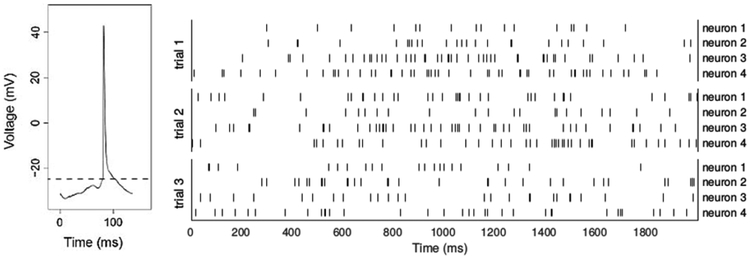
Action potential and spike trains. The left panel shows the voltage drop recorded across a neuron’s cell membrane. The voltage fluctuates stochastically, but tends to drift upward, and when it rises to a threshold level (dashed line) the neuron fires an action potential, after which it returns to a resting state; the neuron then responds to inputs that will again make its voltage drift upward toward the threshold. This is often modeled as drifting Brownian motion that results from excitatory and inhibitory Poisson process inputs (Tuckwell 1988; Gerstein and Mandelbrot 1964). The right panel shows spike trains recorded from 4 neurons repeatedly across 3 experimental replications, known as trials. The spike times are irregular within trials, and there is substantial variation across trials, and across neurons.

Figure 2

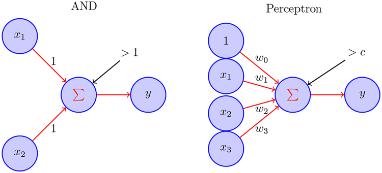
In the left diagram, McCulloch-Pitts neurons x₁ and x₂ each send binary activity to neuron y using the rule y = 1 if x₁ + x₂ > 1 and y = 0 otherwise; this corresponds to the logical AND operator; other logical operators NOT, OR, NOR may be similarly implemented by thresholding. In the right diagram, the general form of output is based on thresholding linear combinations, i.e., y =1 when ∑w_ix_i >c and y = 0 otherwise. The values w_i are called synaptic weights. However, because networks of perceptrons (and their more modern artificial neural network descendents) are far simpler than networks in the brain, each artificial neuron corresponds conceptually not to an individual neuron in the brain but, instead, to large collections of neurons in the brain.

Figure 3

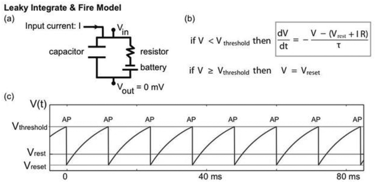
(a) The LIF model is motivated by an equivalent circuit. The capacitor represents the cell membrane through which ions cannot pass. The resistor represents channels in the membrane (through which ions can pass) and the battery a difference in ion concentration across the membrane. (b) The equivalent circuit motivates the differential equation that describes voltage dynamics (gray box). When the voltage reaches a threshold value (V_threshold), it is reset to a smaller value (V_reset). In this model, the occurrence of a reset indicates an action potential; the rapid voltage dynamics of action potentials are not included in the model. (c) An example trace of the LIF model voltage (blue). When the input current (I) is large enough, the voltage increases until reaching the voltage threshold (red horizontal line), at which time the voltage is set to the reset voltage (green horizontal line). The times of reset are labeled as “AP”, denoting action potential. In the absence of an applied current (I = 0) the voltage approaches a stable equilibrium value (V_rest).

Figure 4

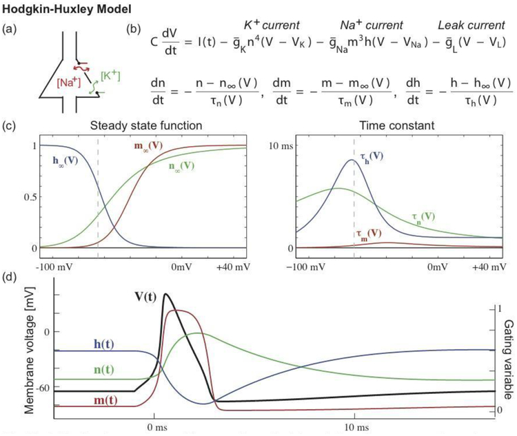
The Hodgkin-Huxley model provides a mathematical description of a neuron’s voltage dynamics in terms of changes in sodium (Na⁺) and potassium (K⁺) ion concentrations. The cartoon in (a) illustrates a cell body with membrane channels through which (Na⁺) and (K⁺) may pass. The model consists of four coupled nonlinear differential equations (b) that describe the voltage dynamics (V), which vary according to an input current (I), a potassium current, a sodium current, and a leak current. The conductances of the potassium (n) and sodium currents (m, h) vary in time, which controls the flow of sodium and potassium ions through the neural membrane. Each channel’s dynamics depends on (c) a steady state function and a time constant. The steady state functions range from 0 to 1, where 0 indicates that the channel is closed (so that ions cannot pass), and 1 indicates that the channel is open (ions can pass). One might visualize these channels as gates that swing open and closed, allowing ions to pass or impeding their flow; these gates are indicated in green and red in the cartoon (a). The steady state functions depend on the voltage; the vertical dashed line indicates the typical resting voltage value of a neuron. The time constants are less than 10 ms, and smallest for one component of the sodium channel (the sodium activation gate m). (d) During an action potential, the voltage undergoes a rapid depolarization (V increases) and then less rapid hyperpolarization (V decreases), supported by the opening and closing of the membrane channels.

Figure 5

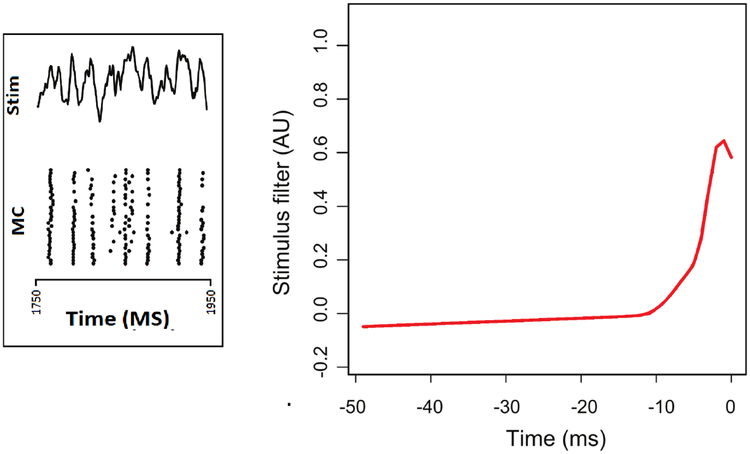
Left panel displays the current (“Stim,” for stimulus, at the top of the panel) injected into a mitral cell from the olfactory system of a mouse, together with the neural spiking response (MC) across many trials (each row displays the spike train for a particular trial). The response is highly regular across trials, but at some points in time it is somewhat variable. The right panel displays a stimulus filter fitted to the complete set of data using model (3), where the stimulus filter, i.e., the function g₀(s), represents the contribution to the firing rate due to the current I(t − s) at s milliseconds prior to time t. Figure modified from (Wang et al. 2015)

Figure 6

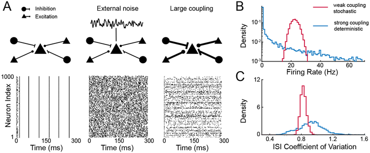
Panel A displays plots of spike trains from 1000 excitatory neurons in a network having 1000 excitatory and 1000 inhibitory LIF neurons with connections determined from independent Bernoulli random variables having success probability of 0.2; on average K = 200 inputs per neuron with no synaptic dynamics. Each neuron receives a static depolarizing input; in absence of coupling each neuron fires repetitively. Left: Spike trains under weak coupling, current J ∝ K⁻¹. Middle: Spike trains under weak couplng, with additional uncorrelated noise applied to each cell. Right: Spike trains under strong coupling, $J\propto K^{-\frac{1}{2}}$. Panel B shows the distribution of firing rates across cells, and panel C the distribution of interspike interval (ISI) coefficient of variation across cells.

References

-
- Abbott LF. 1999. Lapicque’s introduction of the integrate-and-fire model neuron (1907). Brain research bulletin 50:303—304 - PubMed
- Abeles M 1982. Role of the cortical neuron: integrator or coincidence detector? Israel journal of medical sciences 18:83—92 - PubMed
- Agresti A 1996. Categorical data analysis, volume 990 New York: John Wiley & Sons
- Albert M, Bouret Y, Fromont M, Reynaud-Bouret P. 2016. Surrogate data methods based on a shuffling of the trials for synchrony detection: the centering issue. Neural Comput. 28:2352–2392 - PubMed
Grants and funding
LinkOut - more resources
Full Text Sources
Research Materials