The relative contribution of color and material in object selection

Abstract

Object perception is inherently multidimensional: information about color, material, texture and shape all guide how we interact with objects. We developed a paradigm that quantifies how two object properties (color and material) combine in object selection. On each experimental trial, observers viewed three blob-shaped objects-the target and two tests-and selected the test that was more similar to the target. Across trials, the target object was fixed, while the tests varied in color (across 7 levels) and material (also 7 levels, yielding 49 possible stimuli). We used an adaptive trial selection procedure (Quest+) to present, on each trial, the stimulus test pair that is most informative of underlying processes that drive selection. We present a novel computational model that allows us to describe observers' selection data in terms of (1) the underlying perceptual stimulus representation and (2) a color-material weight, which quantifies the relative importance of color vs. material in selection. We document large individual differences in the color-material weight across the 12 observers we tested. Furthermore, our analyses reveal limits on how precisely selection data simultaneously constrain perceptual representations and the color-material weight. These limits should guide future efforts towards understanding the multidimensional nature of object perception.

Fig 1. Vision is used to judge object properties.

A. Color differentiates between ripe and unripe tomatoes. B. Glossiness differentiates between paper and ceramic cups. C. A carefully crafted case where vision misleads us about material. What looks like a rubber basketball is in fact a sculpture made of glass, created by Chris Taylor. (Photography sources: A: Courtesy of Jeroen van de Peppel. B: Courtesy of Michael Eisenstein. C: Courtesy of Chris Taylor; http://www.craftadvisory.com).

Fig 2. Example trial in the experiment.

The observer viewed three rendered scenes, each containing a blob-shaped object. The object in the center scene was the target object. The objects in the left and the right scenes were the test objects. The observer selected which of the two test objects was most similar to the target. The two tests differed from the target in color and/or material (see text for details). In the example shown, both tests differ from the target in both color and material (left test, C₊₃M_-3, is more glossy and bluer; right test C_-3M₊₃ is more matte and greener; see Fig 3 for explanation of stimulus coding conventions).

Fig 3. Stimulus examples.

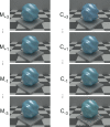
Left column shows stimuli that have the same color as the target and vary only in material: these illustrate variation on the material dimension, from most glossy (M_-3) to most matte (M₊₃). The numerical labels indicate the nominal degree of color/material difference from the target, which is labeled C₀M₀. Only large (M_-3, M₊₃) and small (M_-1, M₊₁) material difference steps are shown. Right column shows stimuli that have the same material as the target and vary only in color: these illustrate variation on the color dimension, from greenest (C_-3) to bluest (C₊₃). Only large (C_-3, C₊₃) and small (C_-1, C₊₁) color difference steps are shown.

Fig 4. Example model solutions.

Results are shown for the best-fitting model for three observers (top row: observer dca; middle row: observer sel; bottom row: observer nkh). Left column. Recovered mean perceptual positions for our test stimuli. The coordinates of the target stimulus are fixed at the origin. Non-target color levels are shown on the x-axis. They are ordered from C_-3 on the left to C₊₃ on the right. Non-target material levels are shown on the y-axis. They are ordered from M_-3 on the bottom to M₊₃ on the top. Different circle colors (black, blue, green, red) indicate different levels of test-to-target difference in color (C) or material (M): zero deviation is plotted in black, small in blue, medium in green and large in red. Points corresponding to differences in the (nominally) negative direction are plotted as open circles, while those corresponding to the (nominally) positive direction are plotted as filled circles. The inferred color-material weight is indicated at the top left. Center column. Measured selection proportions are plotted against proportions predicted by the model. The area of each data point is proportional to the number of trials run for the corresponding stimulus pair. One probability is plotted for each stimulus pair. Only data for stimulus pairs that were presented more than once are shown. Right column. Color-material trade-off functions predicted by the model solution (see main text). Measured probabilities for a subset of trials shown in the experiment are plotted against predicted probabilities. Symbol color matches the corresponding color-material trade-off function. Data corresponding to a prediction are plotted if more than 10 trials were run for the stimulus pair. Open circles correspond to dashed-lines (M_-3, M_-2, M_-1) and filled circles correspond to solid-lines (M₊₃, M₊₂, M₊₁).

Fig 5. Color-material weight varies across observers.

For each observer, the figure shows the color-material weight inferred from the best-fitting model variant (green circles). Which variant was best for each observer is provided in Table 1. Error-bars indicate the central 68% confidence interval (confidence range corresponds to the size of 1 SEM for a Gaussian distribution), obtained via bootstrapping. Black x symbols show the mean of the bootstrapped weights. Red squares show the weight inferred from the best-fitting model for the alternative distance metric.

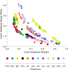
Fig 6. Color-material slope ratio is inversely related to the color-material weight.

Top panel. For each observer we plot the color-material slope ratio against the inferred weight for each bootstrap iteration (see text). Different observers are plotted in different colors. Black open circles plot the color/material slope ratio against the color-material weight inferred from the best-fitting model (full data set) and are superimposed over the corresponding observer’s data for different iterations. Bottom panel. Legend showing color-to-observer mapping used in the top panel to help the reader connect the data shown here with those shown in Table 1 and Figs 4 and 5.

Fig 7. Inferred vs. simulated weights for three simulated observers.

The simulated observer color-material weights are shown in green (identical to those shown for corresponding observers in Fig 5) while the inferred weights from the simulated data are shown in black. Error-bars show the central 68% confidence interval, obtained via bootstrapping for real observers (in green) and simulated observers (in black).

Fig 8. Recovered mean perceptual stimulus positions for three simulated observers.

The stimulus positions on the color dimension are plotted in the left panel, while the positions on the material dimensions are plotted in the right panel. In both plots, recovered positions are plotted against simulated positions. The positive diagonal indicates the identity line and different colors indicate different simulated observers (gfn is shown yellow, lza in violet, nkf in green).

References

1. Wandell BA. Foundations of Vision. Sunderland, MA: Sinauer; 1995.
1. Rodieck RW. The First Steps in Seeing. Sunderland, Mass: Sinauer; 1998.
1. Olkkonen M, Ekroll V. Color Constancy and Contextual Effects on Color Appearance In: Kremers J, Baraas RC, Marshall NJ, editors. Human Color Vision. Cham: Springer International Publishing; 2016. p. 159–88.
1. Foster DH. Color constancy. Vision Research. 2011;51:674–700. 10.1016/j.visres.2010.09.006 - DOI - PubMed
1. Chadwick AC, Kentridge RW. The perception of gloss: A review. Vision Research. 2015;109:221–35. 10.1016/j.visres.2014.10.026 - DOI - PubMed
Publication types