. 2019 Apr 19;364(6437):255.
doi: 10.1126/science.aav7893. Epub 2019 Apr 18.

Spontaneous behaviors drive multidimensional, brainwide activity

Affiliations

Spontaneous behaviors drive multidimensional, brainwide activity

Carsen Stringer et al. Science. .

Abstract

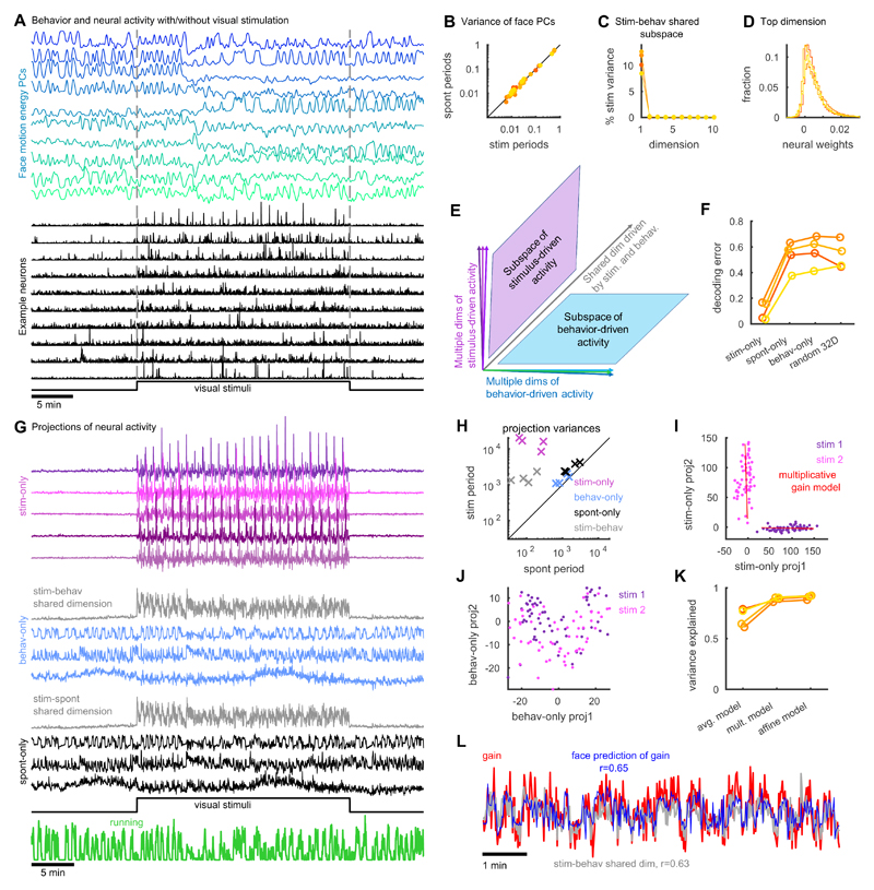
Neuronal populations in sensory cortex produce variable responses to sensory stimuli and exhibit intricate spontaneous activity even without external sensory input. Cortical variability and spontaneous activity have been variously proposed to represent random noise, recall of prior experience, or encoding of ongoing behavioral and cognitive variables. Recording more than 10,000 neurons in mouse visual cortex, we observed that spontaneous activity reliably encoded a high-dimensional latent state, which was partially related to the mouse's ongoing behavior and was represented not just in visual cortex but also across the forebrain. Sensory inputs did not interrupt this ongoing signal but added onto it a representation of external stimuli in orthogonal dimensions. Thus, visual cortical population activity, despite its apparently noisy structure, reliably encodes an orthogonal fusion of sensory and multidimensional behavioral information.


Conflict of interest statement

Declaration of interests

The authors declare no competing interests.

Figures

Figure 1
Figure 1. Structured ongoing population activity in visual cortex.
(A,B) Two-photon calcium imaging of 10,000 neurons in visual cortex using multi-plane resonance scanning of 11 planes spaced 35 μm apart. (C) Distribution of pairwise correlations in ongoing activity, computed in 1.2 second time bins (yellow). Gray: distribution of correlations after randomly time-shifting each cell’s activity. (D) Distribution of pairwise correlations for each recording (showing 5th and 95th percentile). (E) First PC versus running speed in 1.2 s time bins. (F) Example timecourse of running speed (green), pupil area (gray), whisking (light green), first principal component of population activity (magenta dashed). (G) Neuronal activity, with neurons sorted vertically by 1st PC weighting, same time segment as F. (H) Same neurons as in G, sorted by a manifold embedding algorithm. (I) Shared Variance Component Analysis (SVCA) method for estimating reliable variance. (J) Example timecourses of SVCs from each cell set in the test epoch (1.2 s bins). (K) Same as J, plotted as scatter plot. Title is Pearson correlation between cell sets: an estimate of that dimension’s reliable variance. (L) % of reliable variance for successive dimensions. (M) Reliable variance spectrum, power law decay of exponent 1.14. (N) % of each SVC’s total variance that can be reliably predicted from arousal variables (colors as in E). (O) Percentage of total variance in first 128 dimensions explainable by arousal variables.
Figure 2
Figure 2. Multi-dimensional behavior predicts neural activity.
(A) Frames from a video recording of a mouse’s face. (B) Motion energy, computed as the absolute value of the difference of consecutive frames. (C) Spatial masks corresponding to the top three principal components (PCs) of the motion energy movie. (D) Schematic of reduced rank regression technique used to predict neural activity from motion energy PCs. (E) Cross-validated fraction of successive neural SVCs predictable from face motion (blue), together with fraction of variance predictable from running, pupil and whisking (green), and fraction of reliable variance (the maximum explainable; gray; cf. Fig. 1L). (F) Top: raster representation of ongoing neural activity in an example experiment, with neurons arranged vertically as in Fig. 1H so correlated cells are close together. Bottom: prediction of this activity from facial videography (predicted using separate training timepoints). (G) Percentage of the first 128 SVCs’ total variance that can be predicted from facial information, as a function of number of facial dimensions used. (H) Prediction quality from multidimensional facial information, compared to the amount of reliable variance. (I) Adding explicit running, pupil and whisker information to facial features provides little improvement in neural prediction quality. (J) Prediction quality as a function of time lag used to predict neural activity from behavioral traces.
Figure 3
Figure 3. Behaviorally-related activity across the forebrain in simultaneous recordings with 8 Neuropixels probes.
(A) Reconstructed probe locations of recordings in three mice. (B) Example histology slice showing orthogonal penetrations of 8 electrode tracks through a calbindin-counterstained horizontal section. (C) Comparison of mean correlation between cell pairs in a single area, with mean correlation between pairs with one cell in that area and the other elsewhere. Each dot represents the mean over all cell pairs from all recordings, color coded as in panel D. (D) Mean correlation of cells in each brain region with first principal component of facial motion. Error bars: standard deviation. (E) Top: Raster representation of ongoing population activity for an example experiment, sorted vertically so nearby neurons have correlated ongoing activity. Bottom: prediction of this activity from facial videography. Right: Anatomical location of neurons along this vertical continuum. Each point represents a cell, colored by brain area as in C,D, with x-axis showing the neuron’s depth from brain surface. (F) Percentage of population activity explainable from orofacial behaviors as a function of dimensions of reduced rank regression. Each curve shows average prediction quality for neurons in a particular brain area. (G) Explained variance as a function of time lag between neural activity and behavioral traces. Each curve shows the average for a particular brain area. (H) Same as G in 200ms bins.
Figure 4
Figure 4. Neural subspaces encoding stimuli and spontaneous/behavioral variables overlap along one dimension.
(A) Principal components of facial motion energy (top) and firing of ten example V1 neurons (bottom). (B) Comparison of face motion energy for each PC during stimulus presentation and spontaneous periods. Color represents recording identity. (C) The percentage of stimulus-related variance in each dimension of the shared subspace between stimulus- and behavior-driven activity. (D) Distribution of cells’ weights on the single dimension of overlap between stimulus and behavior subspaces. (E) Schematic: stimulus- and behavior-driven subspaces are orthogonal, while a single dimension (gray; characterized in panels C,D) is shared. (F) Stimulus decoding analysis for 32 natural image stimuli from 32 dimensions of activity in the stimulus-only, behavior-only, and spontaneous-only subspaces, together with randomly-chosen 32-dimensional subspaces. Y-axis shows fraction of stimuli that were identified incorrectly. (G) Example of neural population activity projected onto these subspaces. (H) Amount of variance of each of the projections illustrated in G, during stimulus presentation and spontaneous periods. Each point represents summed variances of the dimensions in the subspace corresponding to the symbol color, for a single experiment. (I) Projection of neural responses to two example stimuli into two dimensions of the stimulus-only subspace. Each dot is a different stimulus response. Red is the fit of each stimulus response using the multiplicative gain model. (J) Same as I for the behavior-only subspace. (K) Fraction of variance in the stimulus-only subspace explained by: constant response on each trial of the same stimulus (avg. model); multiplicative gain that varies across trials (mult. model); and a model with both multiplicative and additive terms (affine model). (L) The multiplicative gain on each trial (red) and its prediction from the face motion PCs (blue).

Comment in

  • Parsing signal and noise in the brain.
    Huk AC, Hart E. Huk AC, et al. Science. 2019 Apr 19;364(6437):236-237. doi: 10.1126/science.aax1512. Epub 2019 Apr 18. Science. 2019. PMID: 31000652 No abstract available.

References

    1. Ringach DL. Current Opinion in Neurobiology. 2009;19:439. - PMC - PubMed
    1. Hoffman K, McNaughton B. Science. 2002;297:2070. - PubMed
    1. Kenet T, Bibitchkov D, Tsodyks M, Grinvald A, Arieli A. Nature. 2003;425:954. - PubMed
    1. Han F, Caporale N, Dan Y. Neuron. 2008;60:321. - PMC - PubMed
    1. Luczak A, Barthó P, Harris KD. Neuron. 2009;62:413. - PMC - PubMed

Publication types

LinkOut - more resources