A Normalization Circuit Underlying Coding of Spatial Attention in Primate Lateral Prefrontal Cortex

Abstract

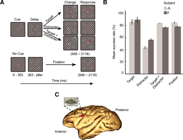
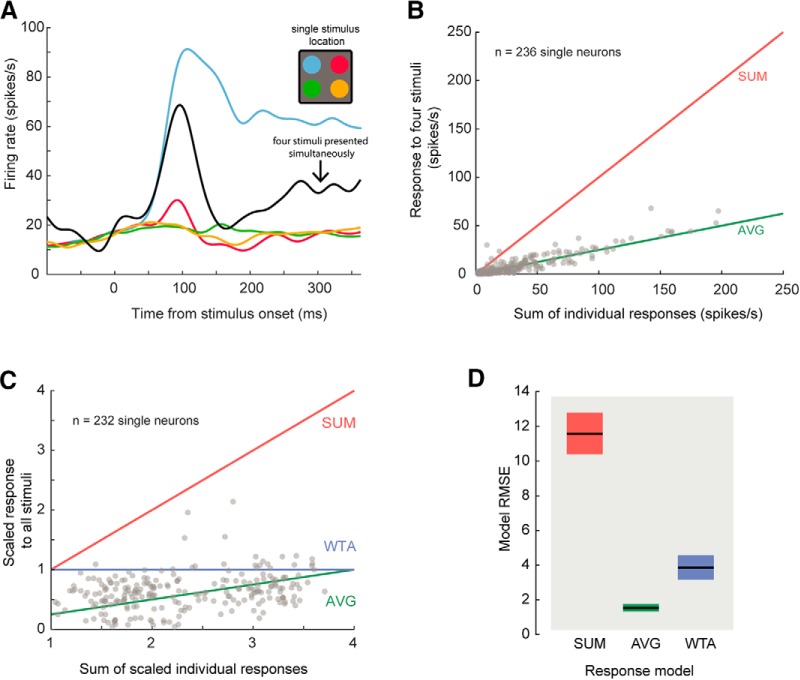
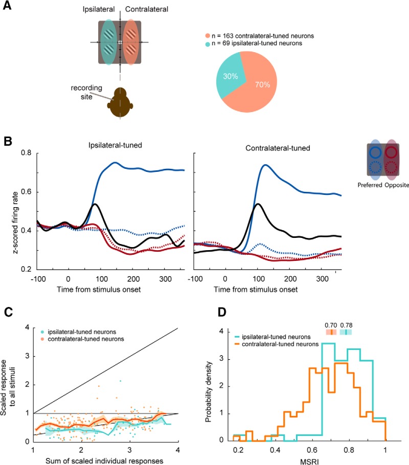
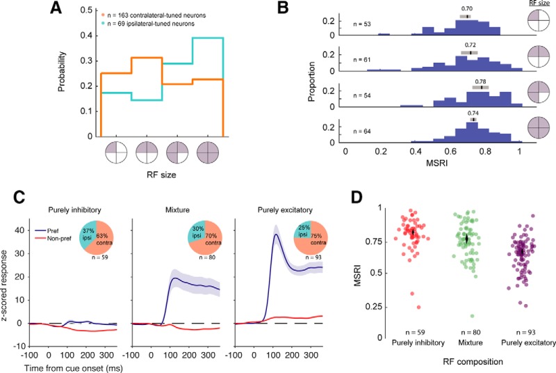
Lateral prefrontal cortex (LPFC) neurons signal the allocation of voluntary attention; however, the neural computations underlying this function remain unknown. To investigate this, we recorded from neuronal ensembles in the LPFC of two Macaca fascicularis performing a visuospatial attention task. LPFC neural responses to a single stimulus were normalized when additional stimuli/distracters appeared across the visual field and were well-characterized by an averaging computation. Deploying attention toward an individual stimulus surrounded by distracters shifted neural activity from an averaging regime toward a regime similar to that when the attended stimulus was presented in isolation (winner-take-all; WTA). However, attentional modulation is both qualitatively and quantitatively dependent on a neuron's visuospatial tuning. Our results show that during attentive vision, LPFC neuronal ensemble activity can be robustly read out by downstream areas to generate motor commands, and/or fed back into sensory areas to filter out distracter signals in favor of target signals.

Keywords: attention; macaque; neurophysiology; normalization; prefrontal cortex.

Figure 1.

Task, methods, and behavior. A, Experimental task design. Top, Attention trials. While the animals maintained fixation on a central point (red color represents gaze location), an initial target cue (Gabor grating at 100% contrast) was randomly presented in one of four quadrants on a computer screen. Three additional stimuli with identical contrast and orientation then appeared in the remaining quadrants of the screen (distracters). The animals needed to covertly attend to the cued stimulus to correctly saccade toward it after it rotated 90° (blue arrows). Bottom, Interleaved fixation trials in which four identical stimuli appeared without an initial cue; animals needed to hold fixation on the central fixation point until the end of the trial. B, Performance of both monkeys in the experimental task (12 recording sessions in Monkey JL; 11 sessions in Monkey F). C, Microelectrode array implantation site: Recordings were collected from area 8a of the left LPFC of each animal.

Figure 2.

Normalization in area 8a. A, Example single unit response to individually-presented stimuli (colored lines) and simultaneously-presented stimuli (black line). B, Responses to multiple versus single stimuli. Each gray point is the sum of a unit’s spiking responses to four individually presented stimuli (x-axis) versus its firing rate when those four stimuli were presented simultaneously (y-axis). The red and green lines are predictions of linear additive (SUM) and averaging (AVG) responses. C, Single unit spiking responses scaled to mean maximal response. Points are the same as in A, but units with super-additive responses (those lying above the red line) were omitted (n = 4). Responses to all stimuli and responses to single stimuli were scaled (divided) by the maximum response to individual stimuli. WTA responses lie on the y = 1 line. D, Bootstrap distributions of RMSEs of each of the three models. The AVG model yielded lowest RMSE (bootstrap t test between Averaging and WTA RMSE; samples; p < 1 × 10⁻⁴). Black lines are mean, and colored boxes are bootstrapped 95% CIs.

Figure 3.

Tuned neural visual responses. A, Individual unit spatial selectivity categorized by visual hemifield relative to recording site. B, Average estimates of continuous firing rates (SDFs) for ipsilateral-tuned (left panel) and contralateral-tuned (right panel) populations. Colored lines are average responses to single stimuli presented in one of four possible quadrants; stimuli were shown inside a unit’s preferred quadrant (i.e., the stimulus which elicited a maximal response; solid blue), in a quadrant adjacent to the unit’s preferred quadrant within the same visual hemifield (dotted blue), adjacent quadrant in the opposite visual hemifield (solid red), or the quadrant located diagonal to the preferred quadrant (dotted red). Black lines are average population responses to these four stimuli when presented simultaneously. C, Same as Figure 2C, but with units classified by their spatial tuning. Bootstrapped moving averages for each tuned population are displayed for visualization purposes (10,000 samples; window size 0.2; step size 0.05). Solid line denotes mean, shaded region denotes 1 SD of the bootstrap sample. D, MSRI for ipsilateral-tuned and contralateral-tuned cells. Bars along top of plot denote median, shaded regions denote central 95% bootstrapped CIs (contralateral-tuned CI [0.67,0.73]; ipsilateral-tuned CI [0.75,0.81]).

Figure 4.

Receptive field properties. A, Distributions of receptive field sizes (number of quadrants) for ipsilateral and contralateral neurons. A quadrant of the visual field was classified as being part of a unit’s receptive field if a singly presented stimulus in that quadrant elicited a response (excitatory or inhibitory) different from pre-stimulus baseline. B, Corresponding MSRI of units with a given receptive field size. Medians (black vertical lines) were computed using 10,000 bootstrap samples, and gray bars indicate the central 95% CIs of the distribution of medians. CIs for top row: [0.65,0.72], second row: [0.66,0.76], third row: [0.73,0.81], and fourth row: [0.71,0.76]. C, Receptive field configurations. Singly presented stimuli may either excite or suppress neuronal activity relative to baseline. Thus, the receptive field of a given neuron can be (1) purely inhibitory, (2) purely excitatory, or (3) a mixture of both. Neuronal responses (z-scored to baseline) were combined for each of the three possible groups. Preferred responses were the responses to stimuli which elicited the greatest response (or the stimuli which elicited the least amount of suppression, in the case of the purely inhibitory RFs). Non-preferred responses are the average response to the three stimuli, excluding the preferred stimulus. Insets show proportion of ipsilateral-tuned and contralateral-tuned cells in each group. D, MSRI of units with RF compositions shown in C. MSRI was greater in units with a greater proportion of inhibitory receptive quadrants. Each dot is one single unit. Dots are horizontally jittered with reduced opacity for clarity. Vertical length of diamonds are 2.5th and 97.5th percentile CIs of the bootstrapped distributions (10,000 samples) of medians. CIs for purely inhibited cells: [0.79,0.83], cells with a mixture of excited and inhibited activity: [0.73,0.79], and purely excited cells: [0.64,0.68].

Figure 5.

Anatomic clustering of spatial tuning. Multielectrode array data from Monkey JL (left column) and Monkey F (right column). A, Multi-unit spatial tuning (ipsilateral or contralateral) on each electrode of the array when using three recording sessions (one per block of 32 electrodes; see Materials and Methods) from each monkey. Black squares are inactive channels, and white squares are channels in which no tuning was present (for details, see Materials and Methods). B, Spatial autocorrelation of tuned clusters on recording array using Moran’s I. Black curves are empirical distributions and gray shaded regions are shuffled 95% null distributions. Although both subjects showed significant clustering at the smallest cluster size, Monkey JL exhibited significant clustering at larger spatial scales than Monkey F. C, Distribution of multi-unit spatial tuning across all recording sessions (12 sessions in Monkey JL, and 11 sessions in Monkey F).

Figure 6.

Ipsilateral and contralateral population attention responses. A, Bootstrapped population average SDFs for ipsilateral (left panel) and contralateral populations (right panel). Attend in, attend out, and fixation trial responses are shown in blue, red. and black, respectively. Attend out trial conditions were averaged across the three non-preferred locations. Single neuron spike trains were trial-averaged, convolved with a Gaussian kernel (15-ms SD), z-scored, and finally averaged within each ipsi/contra population. B, Comparison between each unit’s response to a single stimulus presented in its RF center during the cue epoch (x-axis) vs its attend in response during the delay epoch when distracters were present (y-axis). Dotted line is when a unit’s attend in response matches its response when presented that stimulus alone (i.e., WTA response). C, The sum of each unit’s responses to individual stimuli (x-axis) versus attend in responses (y-axis); x-coordinates of each point are identical to those in Figure 2B. D, RMSE for WTA and AVG models during attend in and attend out conditions for ipsilateral-tuned and contralateral-tuned units. For attend out conditions, we used trials where the animals were attending to the quadrants adjacent to a given unit’s preferred quadrant and located in the opposite hemifield. We found similar results using attend out responses for the remaining two quadrants (i.e., either attending to the quadrant diagonal to the preferred quadrant, or the quadrant adjacent to the preferred quadrant and in the same hemifield) as well. RMSE for SUM models were omitted for clarity due to being much greater in magnitude compared to AVG and WTA model RMSE.

Figure 7.

Single neuron characterization of attention dynamic responses. Bootstrapped average population WTA index (y-axis) over time (x-axis) for (A) attend in and (B) attend out conditions. We computed linear regression slopes (arrows) for the decaying, and sustained attention portions of the curves during time bins denoted by gray bars on the x-axis. Shaded error bars are 1 SD. Each line was computed using 10,000 bootstrap samples.

Figure 8.

Temporal dynamics of attention. A, State space trajectories. Average activity across contralateral neurons (x-axis) is plotted against average activity across ipsilateral neurons (y-axis) for each point in time (z-axis) and averaged within each trial condition. Colored lines are average activity during the four possible attention trial conditions, and the black line is the average activity during the Fixation trial condition in which no cue was presented. B, Euclidean distance through time of each average attention trial condition trajectory (colored) from the fixation trajectory in A. Dashed black line is the average of the four conditions. A linear regression slope was computed for the dashed line during the latter portion of the delay epoch (gray time bin). C, Time-evolving Euclidean distance of each attention trial condition’s delay epoch activity (i.e., activity after distracter onset) from its respective mean activity during the cue epoch. Dashed line is the average of the four conditions. D, Pairwise Euclidean distance between each attention trial trajectory in A. Dashed line is the average of all the pairwise comparisons. Comparisons were made between conditions where the animal attended to the top left (tl), top right (tr), bottom left (bl), or bottom right (br) quadrants of the screen. A linear regression slope was computed during the latter portion of the delay epoch (gray time bin).

Figure 9.

WTA decoding with sustained attention. A, Linear classifier using a pseudopopulation of 232 single unit firing rates trained on the latter 300 ms of the cue epoch, then tested on: (1) firing rates computed in a 300-ms time window (pink shaded error bar, using firing rates integrated over gray time bin shown along x-axis), and (2) dynamic, trailing moving windows during the delay epoch (window = boxcar with width 25 ms; step size = 25 ms). Solid lines are mean classification accuracy, and shaded error is 1 SD of entire bootstrapped sample. Classification accuracy slowly increased after recovery from transient activity after distracter onset (linear regression computed on dynamic classification accuracy during time bin denoted by gray shaded region) with a slope of 0.02 ± 0.01 ms⁻¹ (mean ± SD; blue arrow). B, Example confusion matrix derived from the final time point of the blue curve in A. Trials in which animals attended toward the ipsilateral hemifield were misclassified more than trials where they were to attend toward the contralateral hemifield (50 ± 3% vs 80 ± 3% correct).

Figure 10.

Ensemble decoding of locus of covert attention during delay epoch. A, Linear classifier trained and tested on 25-ms trailing windows stepped by 25 ms during the delay epoch of the task. Bootstrapped average classification accuracies using ensembles comprising exclusively the ipsilateral-tuned population (blue) or contralateral-tuned population (orange), or an ensemble comprising both populations (black). Shaded error bars are 1 SD of the entire bootstrap sample. B–D, Confusion matrices for the ipsilateral-tuned, contralateral-tuned and full population classifiers derived from the final time points of the curves in A.

Figure 11.

Hypothetical normalization circuit in the LPFC. The diagram illustrates a top view of the left and right hemispheres of a macaque monkey brain. The arrows illustrate the origin of excitatory inputs into the pools of contralateral and ipsilateral neurons. The arrows illustrate excitatory (red) or inhibitory (blue) connections between pools of neurons. Triangles are individual units. The colors indicate their spatial preference.

References

1. Alvarez GA, Gill J, Cavanagh P (2012) Anatomical constraints on attention: hemifield independence is a signature of multifocal spatial selection. J Vis 12:9–9. 10.1167/12.5.9 - DOI - PMC - PubMed
1. Armstrong KM, Chang MH, Moore T (2009) Selection and maintenance of spatial information by frontal eye field neurons. J Neurosci 29:15621–15629. 10.1523/JNEUROSCI.4465-09.2009 - DOI - PMC - PubMed
1. Boulay CB, Pieper F, Leavitt M, Martinez-Trujillo J, Sachs AJ (2016) Single-trial decoding of intended eye movement goals from lateral prefrontal cortex neural ensembles. J Neurophysiol 115:486–499. 10.1152/jn.00788.2015 - DOI - PMC - PubMed
1. Boynton GM (2009) A framework for describing the effects of attention on visual responses. Vision Res 49:1129–1143. 10.1016/j.visres.2008.11.001 - DOI - PMC - PubMed
1. Britten KH, Heuer HW (1999) Spatial summation in the receptive fields of MT neurons. J Neurosci 19:5074–5084. 10.1523/JNEUROSCI.19-12-05074.1999 - DOI - PMC - PubMed
Publication types
LinkOut - more resources