. 2019 Jan;124(1):403-431.
doi: 10.1029/2018JC014059. Epub 2019 Jan 21.

Southern Ocean Biogeochemical Float Deployment Strategy, With Example From the Greenwich Meridian Line (GO-SHIP A12)

Affiliations

Southern Ocean Biogeochemical Float Deployment Strategy, With Example From the Greenwich Meridian Line (GO-SHIP A12)

L D Talley et al. J Geophys Res Oceans. 2019 Jan.

Abstract

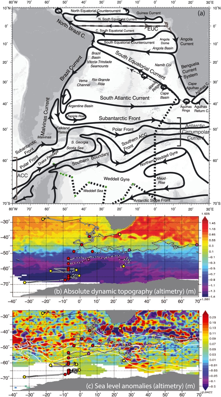
Biogeochemical Argo floats, profiling to 2,000-m depth, are being deployed throughout the Southern Ocean by the Southern Ocean Carbon and Climate Observations and Modeling program (SOCCOM). The goal is 200 floats by 2020, to provide the first full set of annual cycles of carbon, oxygen, nitrate, and optical properties across multiple oceanographic regimes. Building from no prior coverage to a sparse array, deployments are based on prior knowledge of water mass properties, mean frontal locations, mean circulation and eddy variability, winds, air-sea heat/freshwater/carbon exchange, prior Argo trajectories, and float simulations in the Southern Ocean State Estimate and Hybrid Coordinate Ocean Model (HYCOM). Twelve floats deployed from the 2014-2015 Polarstern cruise from South Africa to Antarctica are used as a test case to evaluate the deployment strategy adopted for SOCCOM's 20 deployment cruises and 126 floats to date. After several years, these floats continue to represent the deployment zones targeted in advance: (1) Weddell Gyre sea ice zone, observing the Antarctic Slope Front, and a decadally-rare polynya over Maud Rise; (2) Antarctic Circumpolar Current (ACC) including the topographically steered Southern Zone chimney where upwelling carbon/nutrient-rich deep waters produce surprisingly large carbon dioxide outgassing; (3) Subantarctic and Subtropical zones between the ACC and Africa; and (4) Cape Basin. Argo floats and eddy-resolving HYCOM simulations were the best predictors of individual SOCCOM float pathways, with uncertainty after 2 years of order 1,000 km in the sea ice zone and more than double that in and north of the ACC.

Keywords: Southern Ocean; biogeochemical floats; carbon cycle; circulation; sea ice; water masses.


Figures

Figure 1
Figure 1
SOCCOM float deployment planning and current status. (a) Deployment cruises for 2014–2020 as proposed in 2013, including international GO‐SHIP sections (http://goship.org; blue), and expected non GO‐SHIP cruises (magenta), with proposed number of floats; these opportunities have evolved significantly. (b) Current status of deployments (Table 1): March 2014 to March 2018. (c) Profile locations through February 2018, with trajectories, representative September sea ice concentration (%) and February sea ice extent from the National Snow and Ice Data Center (Maslanik & Stroeve, 1999, updated daily), and 3,000‐m isobath (light brown) from etopo2 (Smith & Sandwell, 1997). Antarctic Circumpolar Current front representations (white in a and b and black in c) from Orsi et al. (1995).
Figure 2
Figure 2
RV Polarstern PS89 (ANT‐XXX/2, 2 December 2014 to 1 February 2015). (a) Planned stations and actual deployments. Red crosses and boxed labels: SOCCOM float deployments, labeled with WMO ID/U. Washington ID (see http://soccom.ucsd.edu/floats/SOCCOM_data_ref.html; Talley et al., 2015). Black dots: PS89 stations (Boebel, 2015). Blue/green dots with white circles: PS89 planned floats/stations prior to cruise (Knust, 2014). Magenta dots: WOCE section A12 (Polarstern ANT‐X/4, 21 May 1992 to 5 August 1992, https://cchdo.ucsd.edu/cruise/06AQANTX_4). (b) Trajectories for SOCCOM floats through May 2017: red (start), yellow (May 2017), magenta (last profile). Black dots: PS89 stations. In both figures, orange bands are 10–20% sea ice concentration in September 2014 (winter, precruise) and February 2015 (summer, postcruise), black curves are representative front locations based on historical hydrographic data (Orsi et al., 1995) and topography is etopo2 (Smith & Sandwell, 1997).
Figure 3
Figure 3
(a) Schematic surface circulation of the South Atlantic, modified from Talley et al. (2011), with planned RV Polarstern PS89 (ANTXXX‐2) track superimposed (dashed and green dots in Weddell Sea). Weddell Sea modifications are from Orsi et al. (1993); Zapiola Rise circulation in Talley et al. has been corrected. (b) Absolute dynamic topography (m) and (c) sea surface height anomalies (m), both from Aviso satellite altimetry on 1 December 2014 (http://las.aviso.altimetry.fr/las/getUI.do), with SOCCOM float tracks as of 28 February 2018 (red: deployment; yellow: current position; magenta: final position), and historical front locations from Orsi et al. (1995; white) (from south to north: SBDY, SACCF, PF, SAF, STF).
Figure 4
Figure 4
(a) Average maximum September mixed layer depth (m) from all Argo profiles 2000–2016, using density threshold criterion, in each 1° latitude/longitude bin (Holte et al., 2017; http://mixedlayer.ucsd.edu). White bins have no September profiles. (b) Wind stress (vectors; N/m2) and negative wind stress curl (× 10−7 N/m3) from NCEP reanalysis 1968–1996 (Kalnay et al., 1996). (c) Surface carbon flux (grams C/m2yr) (Takahashi et al., 2009). Positive is flux out of the ocean (outgassing). (d) Annual mean surface buoyancy flux converted to equivalent heat flux (W/m2), summed from (e) annual mean surface heat flux and (f) annual mean freshwater flux converted to equivalent heat flux, all from Large and Yeager (2009), following Cerovecki et al. (2011). Positive values are flux into the ocean, reducing density. In all panels: RV Polarstern PS89 float deployment locations (red), location at end of February 2018 (yellow), or final location (large magenta). Climatological frontal locations (white) from Orsi et al. (1995) (from south to north: SBDY, SACCF, PF, SAF, STF).
Figure 5
Figure 5
Vertical sections along World Ocean Circulation Experiment (WOCE) Hydrographic Programme (WHP) section A12 from the WHP Atlantic Atlas (Koltermann et al., 2011), annotated with topographic and frontal features: (a) potential temperature (°C), (b) salinity, (c) neutral density (kg/m3), (d) nitrate (μmol/kg), (e) oxygen (μmol/kg), and (f) dissolved inorganic carbon (μmol/kg). WHP section A12 was occupied 21 May 1992 to 5 August 1992. Station positions are shown in Figure 2a. The 2014–2015 PS89 section followed a similar track, with differences at the northern end. SOCCOM float latitudes are shown in panel (a), at 1,000 m, which is the float parking depth.
Figure 6
Figure 6
(a–c) Float trajectory maps, each panel including SOCCOM PS89 trajectories (heavy lines with white core) through October 2017: (a) Argo float trajectories that pass through 2 × 2° range of actual PS89 float deployment, tracked to maximum time of SOCCOM trajectory as of October 2017, or until they die if trajectory is shorter. (b) SOSE‐simulated float trajectories. The cluster at each SOCCOM float deployment location represents 365 synthetic floats, released one per day for a year, starting 1 January 2005 and followed for 3 years. (Supporting information Figure S1b shows the SOSE simulation used for planning purposes, including all PS89 stations, and a different release protocol.) (c) HYCOM‐simulated float trajectories, for 2 years, starting at each planned station location. (d–f) Postdeployment trajectory analysis, using SOCCOM float trajectories for November 2014 to February 2017. RMS difference distance between actual SOCCOM float trajectories (UW ID numbers) and (d) Argo float trajectories, (e) SOSE‐simulated floats, and (f) HYCOM‐simulated floats. (As float 5904473/9260 location was added during the cruise, there is no associated HYCOM simulation.) See also supporting information Figures S1 and S2.
Figure 7
Figure 7
Time series and profiles from two representative SOCCOM floats deployed from PS89 ANT‐XXX/2 (WMO ID 5904469/UW ID 9096—Southern Zone; WMO ID 5904472/UW ID 9275—Antarctic Slope Front): (a, g) potential temperature (°C), (b, h) oxygen (μmol/kg), (c, i) nitrate (μmol/kg), (d, j) potential temperature versus salinity, (e, k) oxygen (μmol/kg), and (f, l) nitrate (μmol/kg). See supporting information Figures S3 and S4 for additional properties from these floats.

Similar articles

Cited by

References

    1. Abernathey, R. P. , Cerovecki, I. , Holland, P. , Newsom, E. , Mazloff, M. , & Talley, L. D. (2016). Water mass transformation by sea ice in the upper branch of the Southern Ocean overturning. Nature Geoscience, 9, 596–601. 10.1038/ngeo2749 - DOI
    1. Ardyna, M. , Claustre, H. , Sallée, J.‐B. , D'Ovidio, F. , Gentili, B. , van Dijken, G. , et al. (2017). Delineating environmental control of phytoplankton biomass and phenology in the Southern Ocean. Geophysical Research Letters, 44, 5016–5024. 10.1002/2016GL072428 - DOI
    1. Arteaga, L. , Haëntjens, N. , Boss, E. , Johnson, K. S. , & Sarmiento, J. L. (2018). Assessment of export efficiency equations in the southern ocean applied to satellite‐based net primary production. Journal of Geophysical Research: Oceans, 123, 2945–2964. 10.1002/2018JC013787 - DOI
    1. Bakker, D. C. E. , Hoppema, M. , Schroder, M. , Geibert, W. , & deBaar H. J. W. (2008). A rapid transition from ice covered CO2‐rich waters to a biologically mediated CO2 sink in the eastern Weddell Gyre. Biogeosciences, 5, 1373–1386. 10.5194/bg-5-1373-2008 - DOI
    1. Balch, W. M. , Drapeau, D. T. , Bowler, B. C. , Lyczskowski, E. , Booth, E. S. , & Alley, D. (2011). The contribution of coccolithophores to the optical and inorganic carbon budgets during the Southern Ocean Gas Exchange Experiment: New evidence in support of the “Great Calcite Belt” hypothesis. Journal of Geophysical Research, 116, C00F06 10.1029/2011JC006941 - DOI