Extensive deep neural networks for transferring small scale learning to large scale systems

Abstract

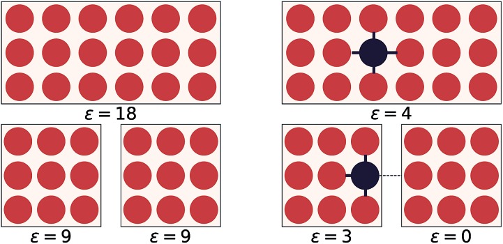
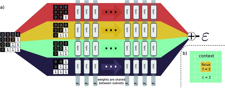
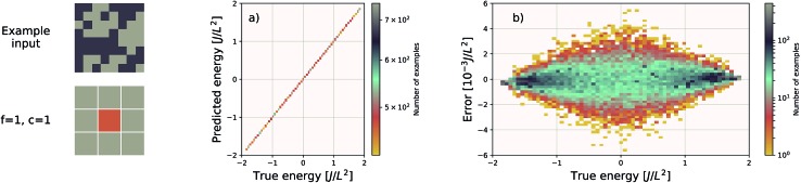
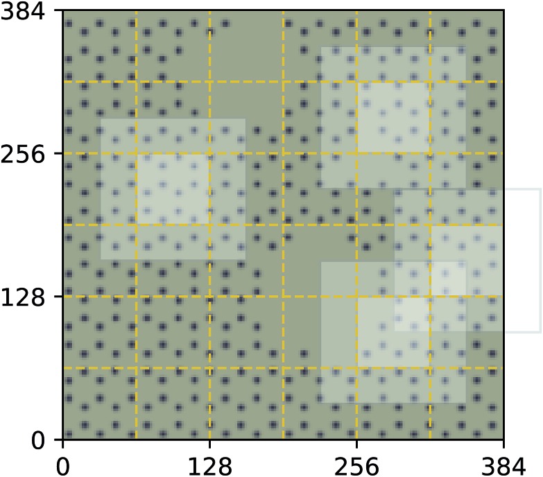
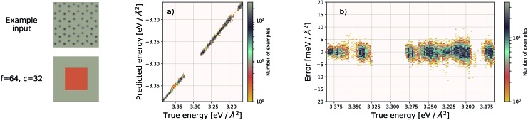
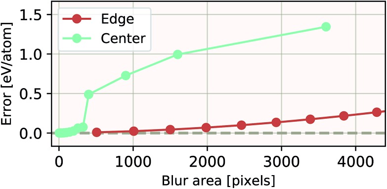
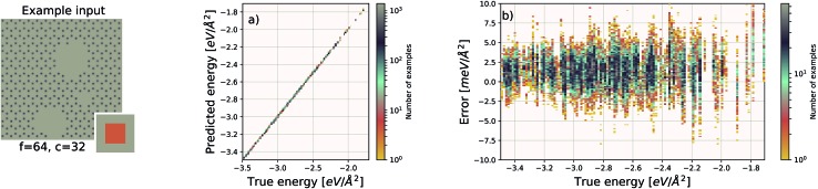
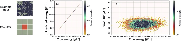
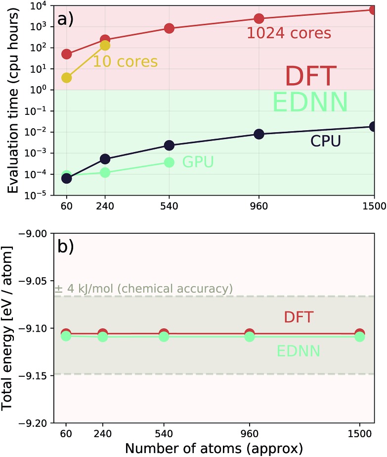
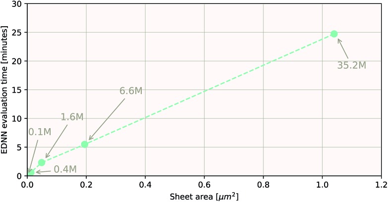
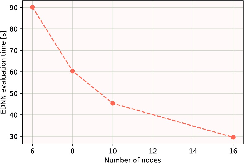
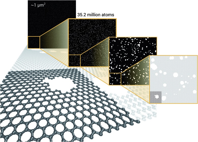
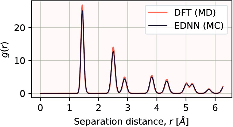
We present a physically-motivated topology of a deep neural network that can efficiently infer extensive parameters (such as energy, entropy, or number of particles) of arbitrarily large systems, doing so with scaling. We use a form of domain decomposition for training and inference, where each sub-domain (tile) is comprised of a non-overlapping focus region surrounded by an overlapping context region. The size of these regions is motivated by the physical interaction length scales of the problem. We demonstrate the application of EDNNs to three physical systems: the Ising model and two hexagonal/graphene-like datasets. In the latter, an EDNN was able to make total energy predictions of a 60 atoms system, with comparable accuracy to density functional theory (DFT), in 57 milliseconds. Additionally EDNNs are well suited for massively parallel evaluation, as no communication is necessary during neural network evaluation. We demonstrate that EDNNs can be used to make an energy prediction of a two-dimensional 35.2 million atom system, over 1.0 μm² of material, at an accuracy comparable to DFT, in under 25 minutes. Such a system exists on a length scale visible with optical microscopy and larger than some living organisms.

Fig. 1. On the left, the counting operator is local and the sum of the operator applied to individual subsystems results in the same answer as the operator applied to the complete system. On the right, the semi-local nearest-neighbour operator (i.e. the count of the number of black-red neighbours) cannot be applied to subsystems separately and then summed.

Fig. 2. An input example is decomposed into four tiles, with each tile consisting of a focus and context region. (a) As a pedagogical example, we expand 4 adjacent tiles comprising a generic binary grid. For this case both the focus and the context are unit width, resulting in 3 × 3 tiles. The tiles are simultaneously passed through the same neural network (i.e. the same weights). The individual outputs are summed, producing an estimate of ε, an extensive quantity. When training, the cost function is assessed after this summation, forcing the weight updates to consider all input tiles simultaneously. In (b), we show an example tile with a focus of f = 2, and a context of c = 2. The optimal selection of f and c depend on the physical length scale of the target (learned) function.

Fig. 3. Performance of an EDNN tasked with learning the energy E operator for the 8 × 8 Ising model. Since E is semi-local (l = 1), f = c = 1 is an optimal configuration. Additional information in the form of a larger context region does not help the network predict values, and in fact makes the training more difficult, as the network must learn to ignore a significant amount of information. (a) Predicted vs. true energies (per spin) for optimal model. (b) Error (predicted – true energy) vs. true energy for optimal EDNN model.

Fig. 4. Decomposition of input image for the quantum mechanical density functional theory calculation using f = 64 and c = 32. Four tiles consisting of a focus region and context region are highlighted. Overlap in the context region is by design and the EDNN must learn to ignore this overlap in the final reduction of the extensive quantity.

Fig. 5. Left: an example graphene sheet. (a) Performance of our EDNN model on a testing set (predicted vs. true). (b) Error ((predicted – true) vs. true) for the EDNN model trained on the total energy as calculated through the density functional theory framework.

Fig. 6. Resilience of an EDNN to the addition of obfuscating Gaussian blur. When a constant amount of information (constant area) within the tiles is blurred, examples that had context area blurred result in more accurate inference than examples that had focus blurred. This is evidence that the EDNN is learning to ignore the context regions.

Fig. 7. Left: an example porous graphene sheet. (a) The true (DFT) vs. predicted (EDNN) total energy in eV Å^–2. The tight clustering along the diagonal indicates the EDNN performs well at predicting the total energy. (b) The error (DFT energy – EDNN energy), in meV Å^–2, is very close to zero.

Fig. 8. An EDNN trained only on 8 × 8 Ising training examples is capable of making accurate predictions of the 128 × 128 Ising model near criticality. While the absolute error is higher at 2.055J/L², the relative error is very small. While it appears the EDNN consistently overpredicts the energy, this is not an effect of large scale inference, but rather that the input configurations are from an energy window where the original EDNN also slightly overpredicted the energy. This is evident when compared to the appropriate region of Fig. 3b.

Fig. 9. A single EDNN was trained on a 12.5 Å × 13 Å unit cell. This trained model was used to make accurate predictions on larger unit cells not present in the training set. (a) The inference time for large systems was about 1 million times smaller than the equivalent density functional theory approach, with CPU evaluation performing better than GPU evaluation on large systems. (b) The resulting energy predictions are consistent within chemical accuracy of 1 kcal mol^–1. The scale of the error can be expected to scale linearly with the size of the system .

Fig. 10. Using the model trained on many small porous graphene sheets, we used a multi-node, distributed TensorFlow implementation to make predictions on large sheets. The model evaluation time scales linearly with the cell area (and thus, under the assumption of homogeneous density, the number of atoms). The annotations refer to the number of atoms in the configuration. The EDNN allows for total energy calculations at DFT accuracy of more than 1.0 μm² of material in 24.7 minutes (Fig. 12). Importantly, the model was trained on a dataset of configurations consisting of only around 500 atoms, and therefore collection of training data does not require accurate simulation of large configurations. All EDNN evaluations were carried out on a 20-node cluster with 28 cores per node.

Fig. 11. Using the model trained on many small porous graphene sheets, we used a multi-node implementation of TensorFlow to perform inference on larger systems. At over 400 000 atoms, we achieve better-than-linear scaling, even with only typical gigabit ethernet interconnect. In theory, since the evaluation of an EDNN is perfectly subdivisible into separate parts, with the only communication cost incurred during the final summation, scaling to large system sizes should be parallel. In practice, overhead is incurred in the distribution of input data, but we achieve impressive scaling nonetheless.

Fig. 12. We demonstrate that EDNNs can be used to make an energy prediction of a two-dimensional 35.2 million atom system, over 1.0 μm² of material, at an accuracy comparable to density functional theory, in under 25 minutes. Additionally, the evaluation of the neural network scales linearly with the number of atoms (assuming relatively homogeneous density), so this evaluation-time estimate can be driven lower with wider hardware configurations. Such a system exists on a length scale visible with optical microscopy and larger than some living organisms.

Fig. 13. The radial distribution functions g(r) plotted for two calculations. The black line is g(r) for a Metropolis Monte Carlo simulation using the EDNN as the energy evaluation function. The orange line is g(r) for a molecular dynamics calculation using density functional theory as the energy evaluation criteria. Since the two methods differ algorithmically, a direct comparison is difficult, but we can see that both methods yield exactly the same peak positions, indicating the EDNN is capable of making predictions at an accuracy suitable for performing physical simulations.

References

1. Chetlur S. and Woolley C., arXiv, 2014, 1–9.
1. Lacey G., Taylor G. W. and Areibi S., arXiv, 2016.
1. Jia Y., Shelhamer E., Donahue J., Karayev S., Long J., Girshick R., Guadarrama S. and Darrell T., arXiv, 2014, 675–678..
1. Silver D., Huang A., Maddison C. J., Guez A., Sifre L., van den Driessche G., Schrittwieser J., Antonoglou I., Panneershelvam V., Lanctot M., Dieleman S., Grewe D., Nham J., Kalchbrenner N., Sutskever I., Lillicrap T., Leach M., Kavukcuoglu K., Graepel T., Hassabis D. Nature. 2016;529:484–489. - PubMed
1. Mnih V., Kavukcuoglu K., Silver D., Rusu A. a., Veness J., Bellemare M. G., Graves A., Riedmiller M., Fidjeland A. K., Ostrovski G., Petersen S., Beattie C., Sadik A., Antonoglou I., King H., Kumaran D., Wierstra D., Legg S., Hassabis D. Nature. 2015;518:529–533. - PubMed