A Stable Visual World in Primate Primary Visual Cortex

Abstract

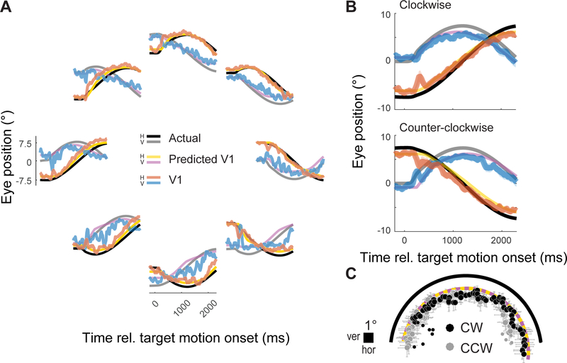
Humans and other primates rely on eye movements to explore visual scenes and to track moving objects. As a result, the image that is projected onto the retina-and propagated throughout the visual cortical hierarchy-is almost constantly changing and makes little sense without taking into account the momentary direction of gaze. How is this achieved in the visual system? Here, we show that in primary visual cortex (V1), the earliest stage of cortical vision, neural representations carry an embedded "eye tracker" that signals the direction of gaze associated with each image. Using chronically implanted multi-electrode arrays, we recorded the activity of neurons in area V1 of macaque monkeys during tasks requiring fast (exploratory) and slow (pursuit) eye movements. Neurons were stimulated with flickering, full-field luminance noise at all times. As in previous studies, we observed neurons that were sensitive to gaze direction during fixation, despite comparable stimulation of their receptive fields. We trained a decoder to translate neural activity into metric estimates of gaze direction. This decoded signal tracked the eye accurately not only during fixation but also during fast and slow eye movements. After a fast eye movement, the eye-position signal arrived in V1 at approximately the same time at which the new visual information arrived from the retina. Using simulations, we show that this V1 eye-position signal could be used to take into account the sensory consequences of eye movements and map the fleeting positions of objects on the retina onto their stable position in the world.

Keywords: computation; electrophysiology; eye position; population coding; primary visual cortex; vision.

Figure 1.. Our sense of a stable visual world arises from retinal images that change with every eye movement.

In the cartoon, a fixed state of the world (i.e., a ball in motion at 5°/s; black arrow) generates three patterns of retinal stimulation (lower panels) under different eye movement scenarios: a fixate-saccade-fixate sequence (purple arrow), and smooth pursuit at 10°/s in opposite directions around a half-circle (green and red arrows). To catch the ball, however, the brain would need to know its true location and program the same set of motor commands, regardless of its appearance on the retina. Note that different coordinate systems are used across panels: world-coordinates (X_w, Y_w) for the object and eye, and retinal coordinates (X_r, Y_r) for the visual images (hereafter, these r and w subscripts are used to indicate the coordinate system of a spatial variable). The object’s trajectory on the retina, o_r(t), is roughly equal to the object’s trajectory in the world, o_w(t), minus the path travelled by the eyes, e_w(t). The brain, however, must make the reverse inference to recover the object’s true trajectory, i.e., o_w(t) = o_r(t) + e_w(t). In this report, we show that V1 neurons represent in parallel both terms on the right side of this equation, and hence implicitly also represent o_w(t).

Figure 2:. Experimental design.

(A) Animals performed a saccade (yellow arrow) or a pursuit task (blue arrow) over a background of flickering noise pixels. The two tasks were interleaved randomly from trial to trial. Filled red circles show the initial and final positions of the target for the 9-o’clock starting position, and the plots show its 2D positon over time in the two tasks. The starting position varied from trial to trial (open circles), with all trials ending at the diametrically opposite position on a virtual circle. Noise pixels are enlarged for illustration. (B) The noise patterns were used to estimate the receptive fields of neurons (See STAR Methods). An example RF is shown for one unit from each animal (M1 and M2), plotted relative to the fovea (red dot). Each image shows the luminance pattern that, on average, caused the unit to generate a spike, as well as an enlarged view of the RF. The units preferred oriented edges (transitions from bright to dark) presented below the fovea (M2) or below and to the left of the fovea (M1). (C) The distribution of receptive fields across all recordings for the two animals. Because the recording array spanned a patch of cortex, units recorded from different electrodes had RFs in slightly different parts of the visual field. Color saturation shows the proportion of recorded units that had RFs that included each location in the display. White areas were outside of the RFs of all recorded units. (D) Example gain-fields for two units, plotted as mean spike counts for 100 ms samples during the fixation epoch (gray shaded region in (A)) at each of nine eye positions (the standard errors of the means are omitted for clarity, but were smaller than the symbols in all cases). Under the assumption of Poisson variability, the fitted regression surfaces provide a generative model relating eye position to spike-count probabilities – a ‘probabilistic gain-field’ (pGF). (E) Population decoding using pGFs. The two leftmost images show the probability of all possible eye positions given observed spike counts of 2 and 6 for units 1 and 2 in (D), respectively. The rightmost image shows the combined probability map for this minimalistic population of two units. The position of the peak (star) represents the maximum likelihood estimate of eye position for this example,[${\widehat{\mathrm{e}}}_{\text{wx}}$,${\widehat{\mathrm{e}}}_{\text{wy}}$]. In practice, the decoded population included all units with gain-fields. See also Figure S1.

Figure 3:. The representation of eye position in V1 is accurate during fixation.

Eye-position was decoded from 100 ms samples of neural activity. Left panel: median decoded eye positions during fixation before (“pre”) and after (“post”) the saccade, compared with the actual fixation positions. Error bars represent the scatter/variability (middle 50% of the distribution) across samples (trials and time). Right panel: decoded positions during the initial fixation phase on pursuit trials. The yellow-purple dashed line is a spline interpolation through the points; it is used in Figure 5 to assess the quality of the decoder during pursuit.

Figure 4:. The representation of eye position updates rapidly with each saccade.

(A) The decoded eye position over time for each saccade direction (red and blue curves), plotted against the average eye trace (black and grey). Plots are arranged spatially according to the starting position (no saccade was required for the central fixation position). Curves -represent the median decoded position and shading represents the variability (middle 50% of distribution) across trials. The grey shaded region indicates the fixation epoch used to build the decoder (i.e. to estimate a pGF for each neuron). (B) The data from (A), averaged over all eight starting positions (after rotating to align their starting positions). Error shading = ±1 STE. (C) The upper panel shows the mean normalized firing rate (see STAR Methods) across the population in response to the flickering background and for a uniform grey background. The lower panel shows the distribution of saccade onset times (relative to the offset of the primary saccades) across all sessions, excluding the primary saccade of the task. Most occur in the wake of the primary saccade. See also Figure S2.

Figure 5:. V1 neurons track the eye during pursuit using the same neural code as during fixation.

(A) Decoded eye position over time for clockwise pursuit, plotted as in Figure 4A, but with the addition of curves (yellow and purple) showing what the decoder performance would look like if the spatial errors in decoder performance seen during fixation (Figure 3) were recapitulated during pursuit. This predicted V1 signal corresponds to the yellow-purple spline shown in Figure 3, but plotted over time (see STAR Methods). (B) As in (A), but averaged over the eight conditions for each pursuit direction. Error shading = ±1 STE. The curves for the predicted signal are mostly obscured by those for the decoded eye, reflecting the close match. (C) The data from (B) plotted in space (black and gray filled circles). Time points before the onset of steady pursuit are plotted as smaller circles. (CW = clockwise, CCW = counter-clockwise). The black curve indicates the true eye position, averaged over clockwise and counter-clockwise directions. The yellow-purple curve indicates the performance predicted on the basis of fixation decoding.

Figure 6.. Population codes for eye position in V1 allow the area as a whole to represent the true locations of objects in the world.

We simulated an observer that localizes objects by combining their instantaneous positions in the V1 retinotopic map with our experimentally measured eye-position signal. The simulated scenarios were identical to our real experiment – including the saccades and pursuit eye movements – but with the addition of an object in linear motion (black arrow) as in Figure 1. The observer’s “perception” (black circles), which indexes the representation of visual space in V1, was accurate even though its projection on the retina differed greatly under different eye movements (coloured arrows). CI shows the compensation index (see STAR Methods) for each of the scenarios. (A) A saccade, identical to that in our real experiment, was performed mid-way through the object’s trajectory. (B) Object motion was viewed during clockwise or counter-clockwise pursuit.

References

1. Kowler E (2011). Eye movements: the past 25 years. Vision Res. 13, 1457–1483. - PMC - PubMed
1. Gur M, and Snodderly DM (1997). Visual receptive fields of neurons in primary visual cortex (V1) move in space with the eye movements of fixation. Vision Res. 3, 257–265. - PubMed
1. Andersen RA, and Buneo CA (2002). Intentional maps in posterior parietal cortex. Annu. Rev. Neurosci 189–220. - PubMed
1. Colby CL, and Goldberg ME (1999). Space and attention in parietal cortex. Annu. Rev. Neurosci 319–349. - PubMed
1. Hartmann TS, Bremmer F, Albright TD, and Krekelberg B (2011). Receptive field positions in area MT during slow eye movements. J. Neurosci 29, 10437–10444. - PMC - PubMed
Publication types