Large-scale molecular phylogeny, morphology, divergence-time estimation, and the fossil record of advanced caenophidian snakes (Squamata: Serpentes)

Abstract

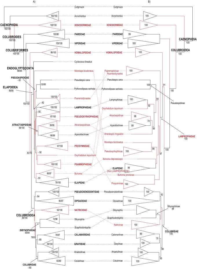
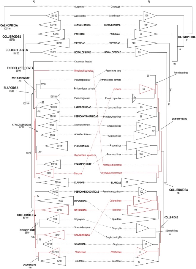
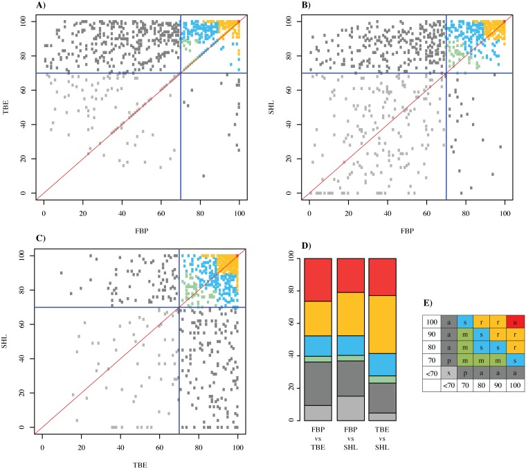
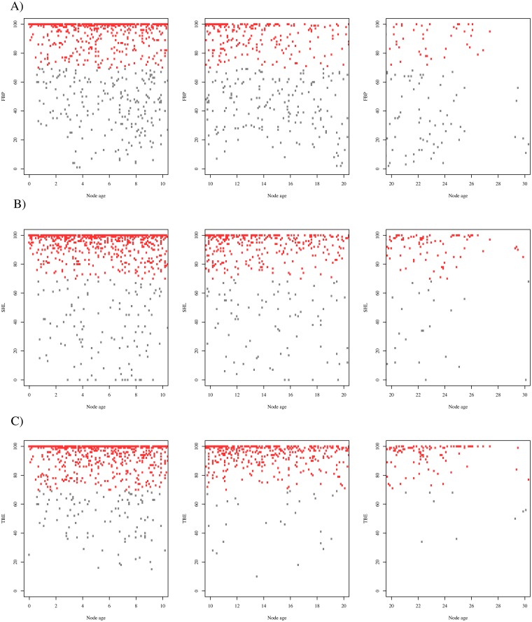
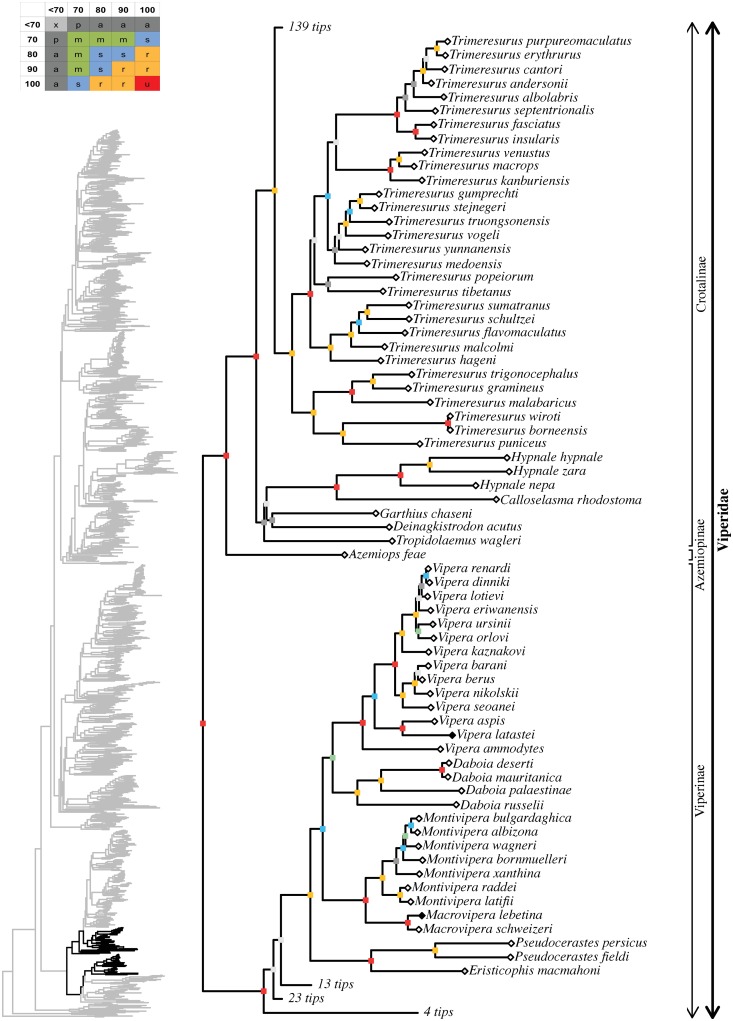
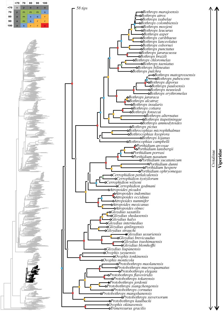
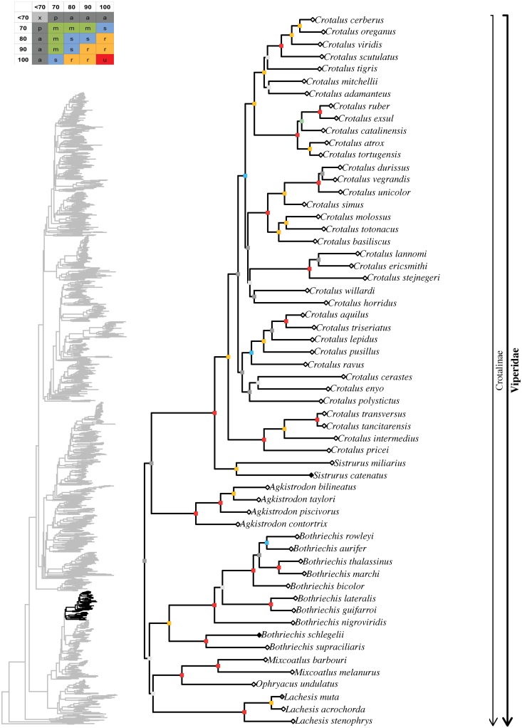
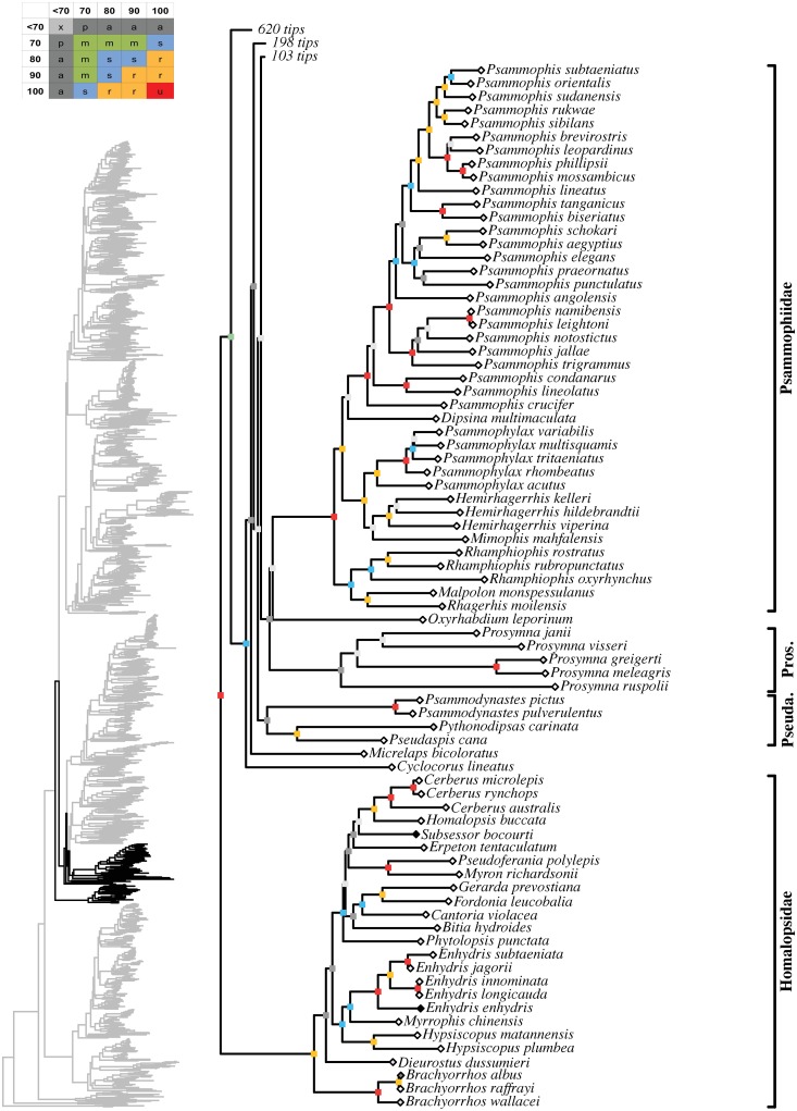
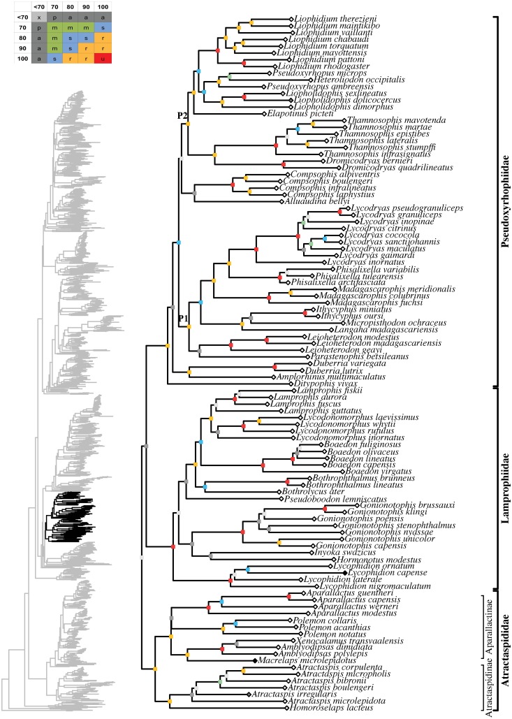
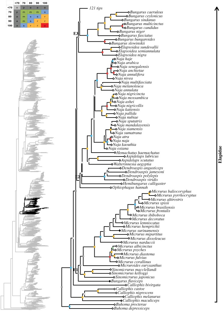
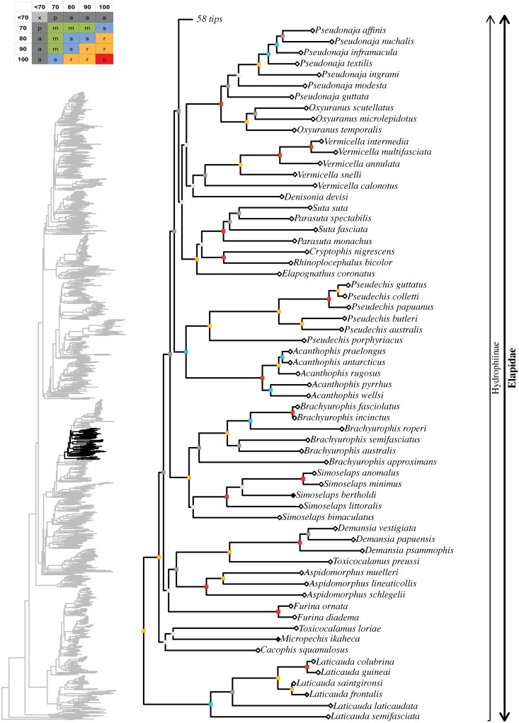
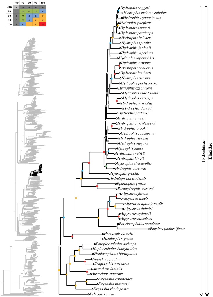
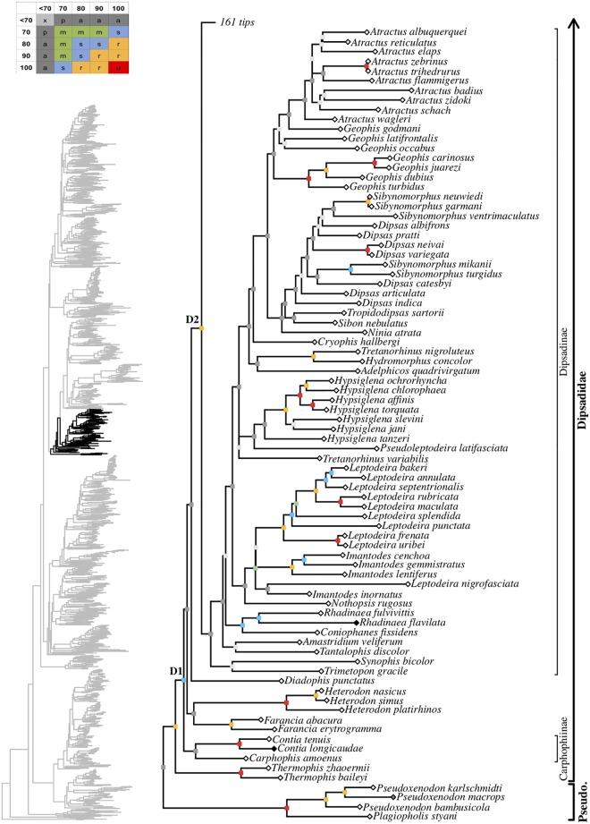
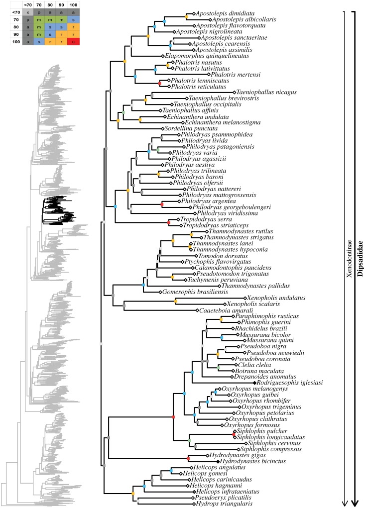
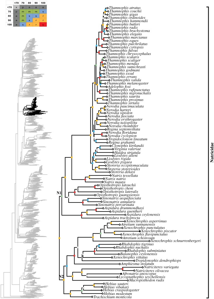
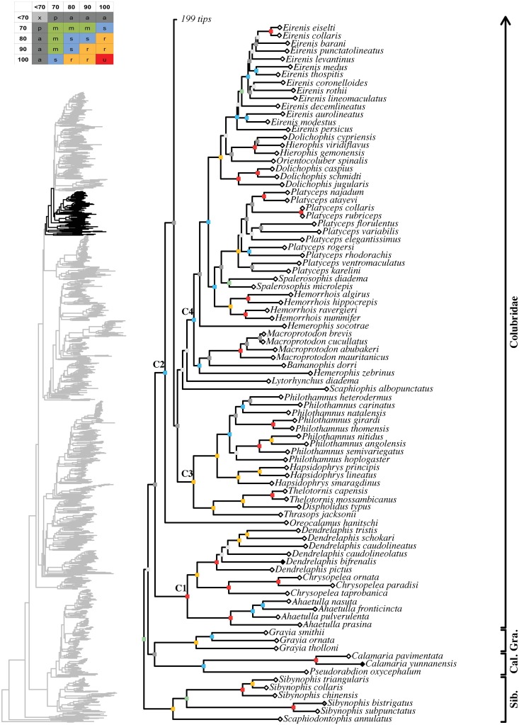
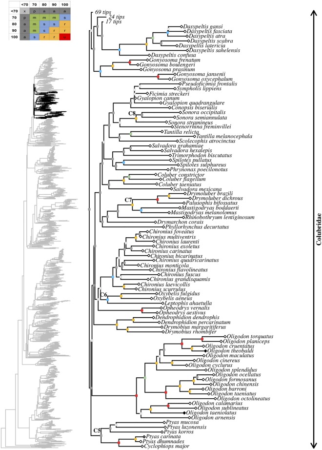
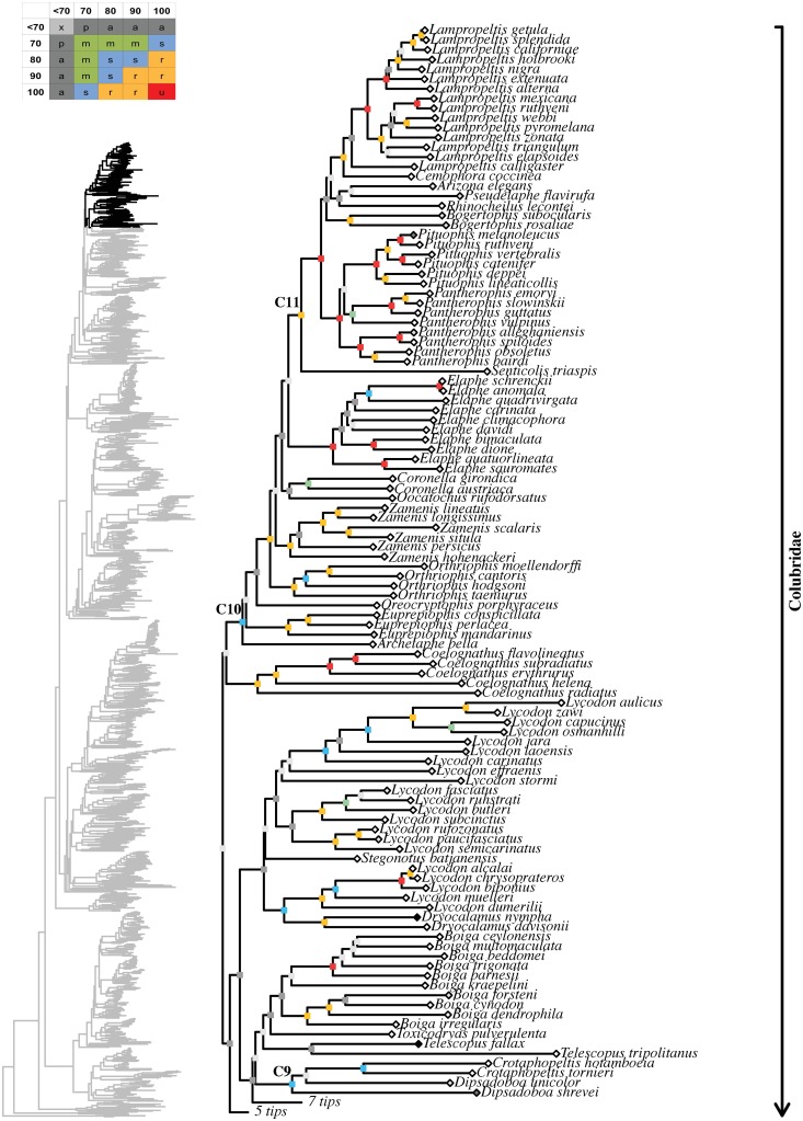
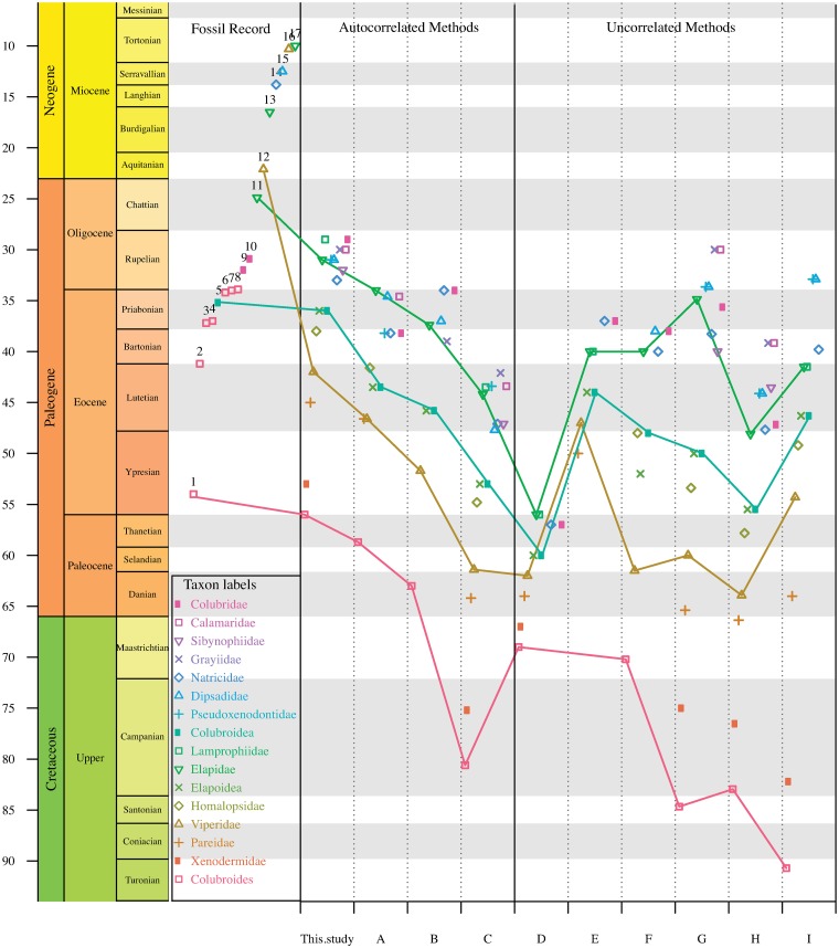
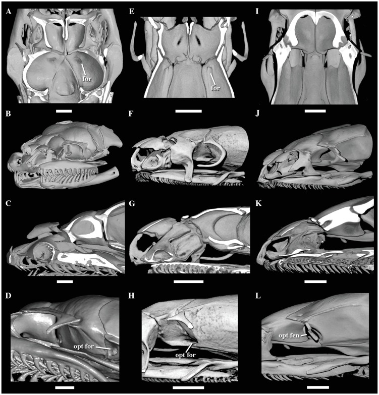
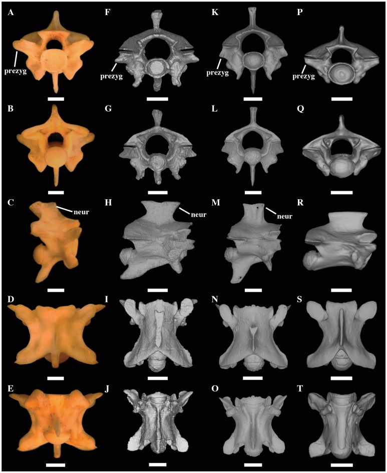
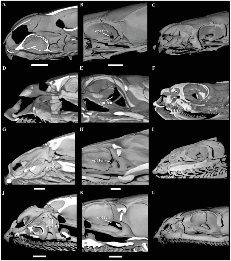
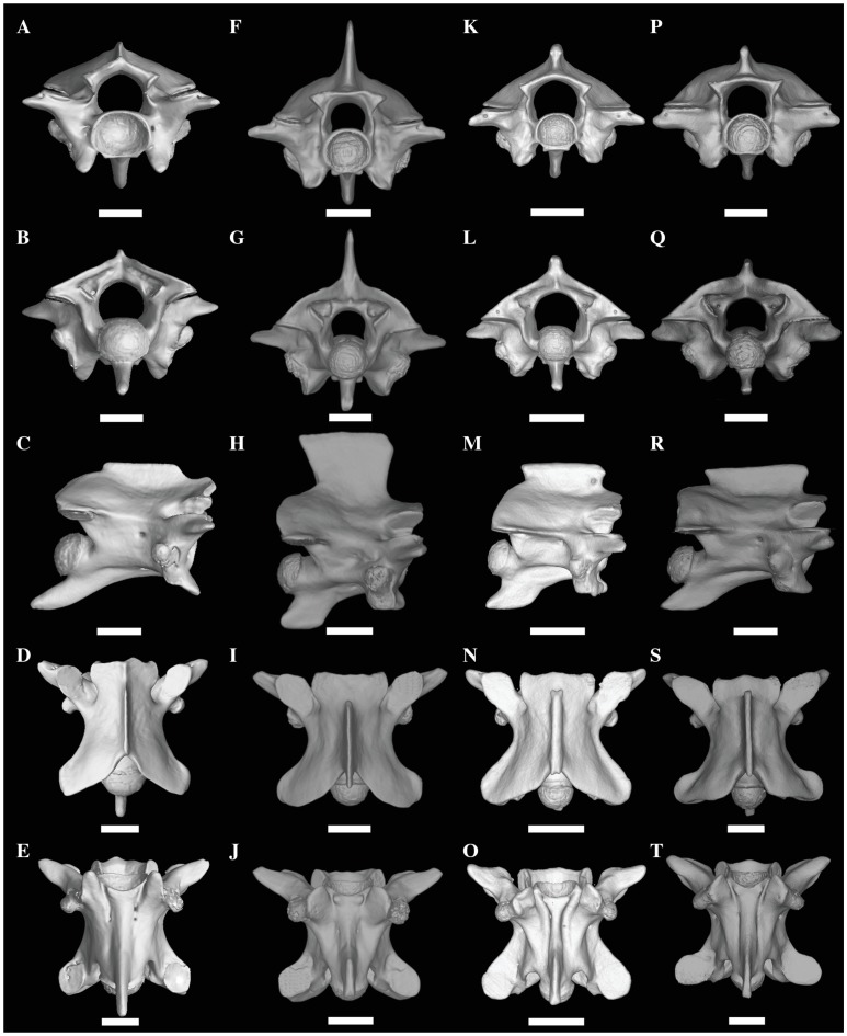
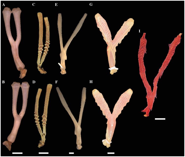
Caenophidian snakes include the file snake genus Acrochordus and advanced colubroidean snakes that radiated mainly during the Neogene. Although caenophidian snakes are a well-supported clade, their inferred affinities, based either on molecular or morphological data, remain poorly known or controversial. Here, we provide an expanded molecular phylogenetic analysis of Caenophidia and use three non-parametric measures of support-Shimodaira-Hasegawa-Like test (SHL), Felsentein (FBP) and transfer (TBE) bootstrap measures-to evaluate the robustness of each clade in the molecular tree. That very different alternative support values are common suggests that results based on only one support value should be viewed with caution. Using a scheme to combine support values, we find 20.9% of the 1265 clades comprising the inferred caenophidian tree are unambiguously supported by both SHL and FBP values, while almost 37% are unsupported or ambiguously supported, revealing the substantial extent of phylogenetic problems within Caenophidia. Combined FBP/TBE support values show similar results, while SHL/TBE result in slightly higher combined values. We consider key morphological attributes of colubroidean cranial, vertebral and hemipenial anatomy and provide additional morphological evidence supporting the clades Colubroides, Colubriformes, and Endoglyptodonta. We review and revise the relevant caenophidian fossil record and provide a time-calibrated tree derived from our molecular data to discuss the main cladogenetic events that resulted in present-day patterns of caenophidian diversification. Our results suggest that all extant families of Colubroidea and Elapoidea composing the present-day endoglyptodont fauna originated rapidly within the early Oligocene-between approximately 33 and 28 Mya-following the major terrestrial faunal turnover known as the "Grande Coupure" and associated with the overall climate shift at the Eocene-Oligocene boundary. Our results further suggest that the caenophidian radiation originated within the Caenozoic, with the divergence between Colubroides and Acrochordidae occurring in the early Eocene, at ~ 56 Mya.

Fig 1. Higher-level caenophidian phylogenies.

Comparison between Maximum-likelihood phylogenetic estimates from (A) the present study and (B) Figueroa et al. [28]. Tips represent commonly recognized families, subfamilies and rogue taxa. Names in red correspond to taxa with distinct phylogenetic positions in the topologies compared. Numbers on each branch and within expanded tips correspond to our and previously reported support values: (A) FBP (left) and SHL (right); (B) FBP. Branches without numbers have support <70%.

Fig 2. Higher-level caenophidian phylogenies.

Comparison between Maximum-likelihood phylogenetic estimates from (A) the present study and (B) Pyron et al. [26]. Tips represent commonly recognized families, subfamilies and rogue taxa. Names in red correspond to taxa with distinct phylogenetic positions in the topologies compared. Numbers on each branch and within expanded tips correspond to our and previously reported support values: (A) FBP (left) and SHL (right); (B) SHL. Branches without numbers have support <70%.

Fig 3. Higher-level caenophidian phylogenies.

Comparison between Maximum-likelihood phylogenetic estimates from (A) the present study and (B) Zheng and Wiens [27]. Tips represent commonly recognized families, subfamilies and rogue taxa. Names in red correspond to taxa with distinct phylogenetic positions in the topologies compared. Numbers on each branch and within expanded tips correspond to our and previously reported support values: (A) FBP (left) and SHL (right); (B) FBP. Branches without numbers have support <70%.

Fig 4. Scatterplots comparing support metrics for internal branches in the Maximum likelihood species-level phylogeny of Colubroides.

A) TBE and FBP B) SHL and FBP C) SHL and TBE, D) Histogram showing the proportion of each category of joint support in each comparison of support metrics, E) Categories of joint support.

Fig 5. Distribution of branch support scores for each node age based on the Maximum likelihood species-level phylogeny of Colubroides.

A) FBP distribution, B) SHL distribution, C) TBE distribution. Red dots represent values greater than 70%; gray dots indicate values smaller than 70%.

Fig 6. Maximum likelihood species-level phylogeny of Colubroides.

Families Xenodermidae, Pareidae, subfamily Viperinae. Skeleton of the complete tree is displayed on the left, with the area of the tree corresponding to the present figure highlighted in black. Colored squares on each node represent bootstrap and SHL values following the categories of combined clade support described in S2 Table and summarized on the upper left corner of the figure. Diamonds on each tip represent the percentage of data generated in this study for each terminal: white, 0%; light grey, between 1% and 50%; dark grey, between 50% and 99%; black, 100%.

Fig 7. Maximum likelihood species-level phylogeny of Colubroides (continued).

Family Viperidae, subfamilies Viperinae, Azemiopinae, Crotalinae.

Fig 8. Maximum likelihood species-level phylogeny of Colubroides (continued).

Family Viperidae, subfamily Crotalinae.

Fig 9. Maximum likelihood species-level phylogeny of Colubroides (continued).

Family Viperidae, subfamily Crotalinae.

Fig 10. Maximum likelihood species-level phylogeny of Colubroides (continued).

Basal Elapoidea, families Homalopsidae, Cyclocoridae, Pseudaspididae, Psammophiidae.

Fig 11. Maximum likelihood species-level phylogeny of Colubroides (continued).

Families Atractaspididae, Lamprophiidae, Pseudoxyrhophiidae.

Fig 12. Maximum likelihood species-level phylogeny of Colubroides (continued).

Family Elapidae.

Fig 13. Maximum likelihood species-level phylogeny of Colubroides (continued).

Family Elapidae (continued).

Fig 14. Maximum likelihood species-level phylogeny of Colubroides (continued).

Family Elapidae (continued).

Fig 15. Maximum likelihood species-level phylogeny of Colubroides (continued).

Families Pseudoxenodontidae and Dipsadidae.

Fig 16. Maximum likelihood species-level phylogeny of Colubroides (continued).

Family Dipsadidae (continued).

Fig 17. Maximum likelihood species-level phylogeny of Colubroides (continued).

Family Dipsadidae (continued).

Fig 18. Maximum likelihood species-level phylogeny of Colubroides (continued).

Family Natricidae.

Fig 19. Maximum likelihood species-level phylogeny of Colubroides (continued).

Families Sibynophiidae, Calamariidae, Grayiidae, and Colubridae.

Fig 20. Maximum likelihood species-level phylogeny of Colubroides (continued).

Family Colubridae (continued).

Fig 21. Maximum likelihood species-level phylogeny of Colubroides (continued).

Family Colubridae (continued).

Fig 22. TreePL calibrated tree showing divergence time estimates for the major families of Colubroides.

Values above branches represent estimated ages in millions of years. Red-shaded vertical bar corresponds to the possible range of the Eocene–Oligocene interval known as the “Grande Coupure”.

Fig 23. Comparative graph showing divergence time estimations for the main clades of Colubroides in some of the main studies published in the last decade.

Numbers near symbols represent the following fossils (see S10 Table for more details): (1) Procerophis sahnii, 54 Mya; (2) Colubroidea Incertae sedis, 41.2 Mya; (3) Colubroidea indet, 37.2 Mya; (4) Renenutet enmerwer, 37 Mya; (5) Colubroidea indet, 35.2 Mya; (6) Nebraskophis sp, 34.2 Mya; (7) Colubrid indet, 34 Mya; (8) Vectophis wardi, 33.9 Mya; (9) Texasophis galbreathi, 32 Mya; (10) Coluber cadurci, 30.9 Mya; (11) Elapidae indet, 24.9 Mya; (12) Vipera cf. V. antiqua, Mya 22.1; (13) Elapidae indet, 16.5 Mya; (14) Natrix longivertebrata, 13.8 Mya; (15) Paleoheterodon tiheni, 12.5 Mya; (16) Sistrurus sp., 10.3 Mya; (17) Incongruelaps iteratus, 10 Mya. Letters represent the following contributions: (A) Burbrink and Pyron [132]; (B) Kelly et al. [22]; (C) Zheng and Wiens [26]; (D) Hsiang et al. (58); (E) Hsiang et al. (58); (F) Wuster et al. [133]; (G) Pyron and Burbrink [134]; (H) Alencar et al. [124]; (I) Vidal et al. [135].

Fig 24. Skulls of Acrochordus granulatus (A-D), Fimbrios klossi (E-H), and Xylophis perroteti (I-L).

Three-dimensional surface and cutaway views based on high resolution X-ray computed tomography. A, E, I, dorsal three-dimensional cutaway views along the frontal axis; B, F, J, oblique three-dimensional surface views; C, G, K, left lateral three-dimensional cutaway views along the sagittal axis; D, H, L, left lateral three-dimensional surface views. Legends: for., optic foramina; opt. fen., optic fenestra. Scale bar = 1mm.

Fig 25. Mid- to posterior trunk vertebrae of Acrochordus javanicus (A-E), Achalinus rufescens (F-J), Fimbrios klossi (K-O), and Pareas sp. (P-T).

Photographs (A-E) and three-dimensional surface views based on high resolution X-ray computed tomography. A, F, K, P, anterior views; B, G, L, Q, posterior views; C, H, M, R, right lateral views; D, I, N, S, dorsal views; E, J, O, T, ventral views. Legends: prezyg., prezygapophysial process; neur., neural spine. Scale bar = 2 mm (A-E) and 1 mm (F-T).

Fig 26. Skulls of Pareas moellendorffi (A-C), Causus rhombeatus (D-F), Enhydris chinensis (G-I), and Afronatrix anoscopa (J-L).

Three-dimensional surface and cutaway views based on high resolution X-ray computed tomography. A, D, G, J left lateral three-dimensional cutaway views along the sagittal axis; B, E, H, K, left lateral three-dimensional surface views; C, F, I, L, oblique three-dimensional surface views. Legends: sept. art., septomaxillary articulation; opt. fen., optic fenestra. Scale bar = 1 mm.

Fig 27. Mid- to posterior trunk vertebrae of Causus difilippi (A-E), Cerberus rynchops (F-J), Cyclocorus lineatus (K-O), and Sinomicrurus macclellandi (P-T).

Three-dimensional surface and cutaway views based on high resolution X-ray computed tomography. A, F, K, P, anterior views; B, G, L, Q, posterior views; C, H, M, R, right lateral views; D, I, N, S, dorsal views; E, J, O, T ventral views. A-E, scale bar = 5 mm; F-J, scale bar = 2mm; K-O, scale bar = 1mm; P-T, scale bar = 1mm.

Fig 28. Hemipenes of Acrochordus javanicus (A-B), Achalinus rufescens (C-D), Pareas monticola (E-F), Asthenodipsas malaccanus (G-H), and Xylophis perroteti (I).

A, C, E, G, sulcate views; B, D, F, H, asulcate views. A, B, E, F, G, H, fully everted and expanded; C, D, fully everted and partially expanded; I, opened through a longitudinal slit, spread flat, and dyed with alizarin red. A-B, scale bar = 5 mm; C-D, scale bars = 2 mm; E-F, scale bar = 1 mm; G-H, scale bar = 1 mm; I, scale bar = 5 mm.

Fig 29. Hemipenes of Porthidum nasutum (A-B), Brachyorrhos albus (C-D), Atractaspis fallax (E-F), Oreocalamus hanitschi (G-H), Grayia ornata (I-J), and Spilotes sulphureus (K-L).

A, C, E, G, I, K, sulcate views; B, D, F, H, J, L, asulcate views. A-L completely everted and expanded. A-D, Scale bars = 5 mm; E-F, scale bar = 10 mm; G-H, scale bar = 5 mm; I-J, Scale bars = 10 mm.

Fig 30. Scanning electron microscopy of maxillary teeth in Acrochordidae, Xenodermidae, Pareidae, and Xylophiinae.

(A) right posterior maxillary teeth of Achalinus formosanus in lingual view; (B) right posterior maxillary teeth of Achalinus rufescens in lingual view; (C) right posterior maxillary teeth of Acrochordus granulosus in labial view; (D) left posterior maxillary teeth of Pareas sp. in lingual view; (E) right posterior maxillary teeth of Xylophis perroteti in labial view. White arrows are pointing to the lateral (labial) and medial (lingual) ridges in the posterior maxillary teeth.

References

1. Underwood G. A contribution to the classification of snakes. London: British Museum of Natural History; 1967.
1. Hoffstetter R. Contribution à l’étude des Elapidae actuels et fossils et de l’ostéologie des ophidiens. Arch Mus Hist Nat. Lyon. 1939;15: 1–75.
1. Haas G. Remarques concernant les relations phylogéniques des diverses familles d’ophidiens fondées sur la différenciation de la musculature mandibulaire. Colloq Int Cent Nat Rech Sci. 1962;104: 215–241.
1. Hoffstetter R, Gayrard Y. Observations sur l’ostéologie et la classification des Acrochordidae (Serpentes). Bull Mus Natl Hist Nat. 1965;36: 677–696.
1. Romer AS. Osteology of the reptiles. Chicago: University of Chicago Press; 1956.
Publication types