Exact hypothesis testing for shrinkage-based Gaussian graphical models

Abstract

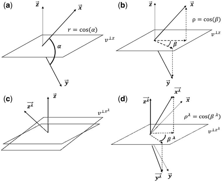
Motivation: One of the main goals in systems biology is to learn molecular regulatory networks from quantitative profile data. In particular, Gaussian graphical models (GGMs) are widely used network models in bioinformatics where variables (e.g. transcripts, metabolites or proteins) are represented by nodes, and pairs of nodes are connected with an edge according to their partial correlation. Reconstructing a GGM from data is a challenging task when the sample size is smaller than the number of variables. The main problem consists in finding the inverse of the covariance estimator which is ill-conditioned in this case. Shrinkage-based covariance estimators are a popular approach, producing an invertible 'shrunk' covariance. However, a proper significance test for the 'shrunk' partial correlation (i.e. the GGM edges) is an open challenge as a probability density including the shrinkage is unknown. In this article, we present (i) a geometric reformulation of the shrinkage-based GGM, and (ii) a probability density that naturally includes the shrinkage parameter.

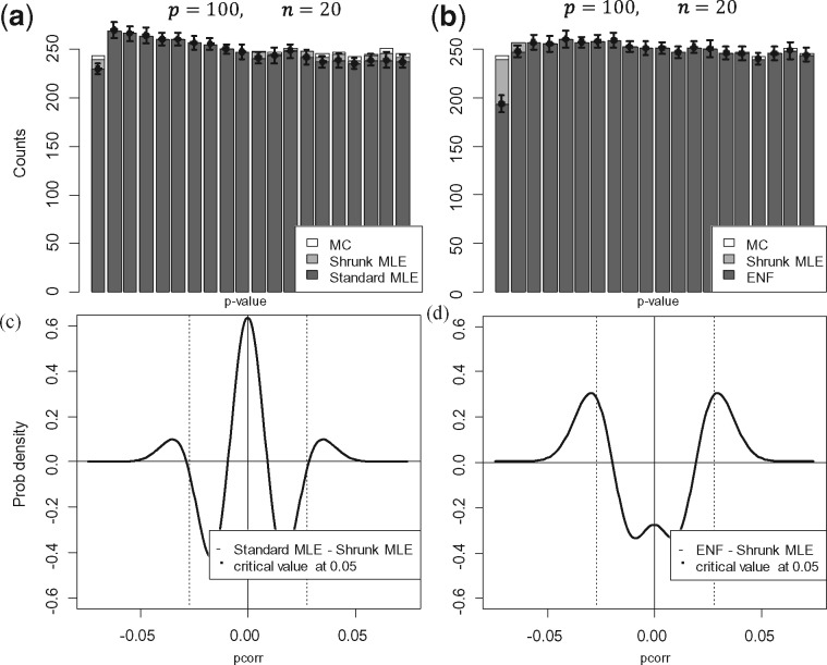
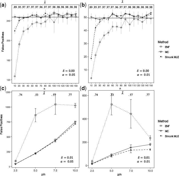
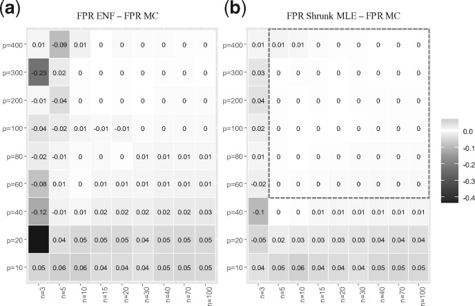
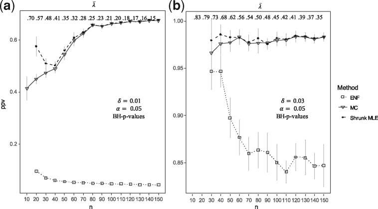
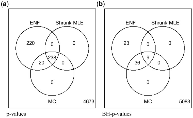
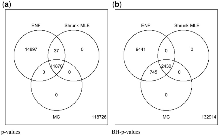
Results: Our results show that the inference using this new 'shrunk' probability density is as accurate as Monte Carlo estimation (an unbiased non-parametric method) for any shrinkage value, while being computationally more efficient. We show on synthetic data how the novel test for significance allows an accurate control of the Type I error and outperforms the network reconstruction obtained by the widely used R package GeneNet. This is further highlighted in two gene expression datasets from stress response in Eschericha coli, and the effect of influenza infection in Mus musculus.

Availability and implementation: https://github.com/V-Bernal/GGM-Shrinkage.

Supplementary information: Supplementary data are available at Bioinformatics online.

Fig. 1.

Geometry of the partial correlation. The vectors ${\displaystyle \overrightarrow{\mathit{x}}}$, ${\displaystyle \overrightarrow{\mathit{y}}}$ and ${\displaystyle \overrightarrow{\mathit{z}}}$ represent the random variables X, Y and Z  in subject space. In Panel (a), the correlation $\mathit{r}$ between X and Y is the cosine of $\alpha$. In Panel (b), the partial correlation between X and Y can be interpreted as the cosine of the angle $\beta$. That is the cosine between the projection of ${\displaystyle \overrightarrow{\mathit{x}}}$ and ${\displaystyle \overrightarrow{\mathit{y}}}$ onto a plane orthogonal to ${\displaystyle \overrightarrow{\mathit{z}}}$. The shrinkage effect consists in that the vectors ${\displaystyle \overrightarrow{\mathit{x}}}$, ${\displaystyle \overrightarrow{\mathit{y}}}$ and ${\displaystyle \overrightarrow{\mathit{z}}}$are transformed to ${\displaystyle \overrightarrow{{\mathit{x}}^{\mathit{\lambda }}}}, {\displaystyle \overrightarrow{{\mathit{y}}^{\mathit{\lambda }}}}$ and ${\displaystyle \overrightarrow{{\mathit{z}}^{\mathit{\lambda }}}}$ such that their lengths remain 1, and only the angles between each other change. In other words, the transformed vectors become less correlated. In Panel (c), the geometrical effect of the shrinkage consists in changing the projection plane ${\mathit{v}}^{\perp \mathit{z}}$ to ${\mathit{v}}^{\perp {\mathit{z}}^{\mathit{\lambda }}}$. In Panel (d), the ‘shrunk’ partial correlation ${\rho }^{\lambda }$ between X and Y is the cosine of the angle ${\beta }^{\lambda }$. That is the cosine between the projections of ${\displaystyle \overrightarrow{{\mathit{x}}^{\mathit{\lambda }}}}$ and ${\displaystyle \overrightarrow{{\mathit{y}}^{\mathit{\lambda }}}}$ onto ${\mathit{v}}^{\perp {\mathit{z}}^{\mathit{\lambda }}}$

Fig. 2.

Probability densities and P-values under$\mathrm{ }{H}_0$. This figure shows a comparison of the standard $f_0\left({\rho }^{\lambda }\right)$ and ‘shrunk’ ${f_0}^{\lambda }\left({\rho }^{\lambda }\right)$ densities, and their P-values under $H_0$. Here Standard MLE denotes $f_0\left({\rho }^{\lambda }\right)$ (i.e. Equation 4) with k obtained via MLE (as in Shrunk MLE). Panel (a) shows the average histogram of P-values obtained with (i) Standard MLE (dark grey), (ii) Shrunk MLE (light grey) and (iii) MC (white) with 15 iterations. Panel (b) replaces Standard MLE by ENF to estimate $k$ in $f_0\left({\rho }^{\lambda }\right)$ (currently used in GeneNet). The bin’s width is set to 0.05; therefore, the first bin represents the amount of significant coefficients at the 5% level. The bin’s height corresponds to the mean over 25 simulations, and the error bars (for ENF) to ±2 SE. It can be seen that the P-values from ENF (dark grey) are not uniformly distributed in [0, 1] under $H_0$. Panels (c) and (d) show the difference $f_0\left({\rho }^{\lambda }\right)-{f_0}^{\lambda }\left({\rho }^{\lambda }\right)$ when $k$ is found via MLE or via ENF, respectively (see Section 2.1). Data were simulated with $p=100$, $n=20$ and $\lambda =$0.94. The critical value at $\alpha =0.05$ (in dashed grey) is estimated by MC (with 100 iterations). It can be seen that $f_0\left({\rho }^{\lambda }\right)$ has larger tails than ${f_0}^{\lambda }\left({\rho }^{\lambda }\right)$

Fig. 3.

False positives. This figure shows the number of FPs obtained with different sample size $n$. The number of FPs are shown in Panels (a) and (b) under $H_0$: no partial correlation (i.e. the percentages of true correlations $\delta$ is zero). Inference is carried out from simulated data for $p$ = 100 and $n$ ranging from 10 to 150 in steps of size 10. The black horizontal line represents the expected number of FPs under$\mathrm{ }{H}_0$, tested at $\alpha$ = 0.05 and$\mathrm{ }0.01$ respectively (i.e. 247.5 for $\alpha$ = 0.05 and 49.5 for $\alpha$=0.01). Panels (c) and (d) show the number of FPs for different proportions $p/n$ when the percentages of non-zero correlations is $\delta$ = 0.01. Here $p$ = 50, 100, 150, 200 and $n$ = 20. Three approaches are compared: ENF (dot with dashed line), Shrunk MLE (square with dotted line), and MC with 15 iterations (triangle with continuous line). Symbols (and bars) represent the average (±2 SE) over 25 repeated simulations. The upper horizontal axis shows the average shrinkage intensity $\stackrel{}{\mathrm{\lambda }}$ rounded to two digits

Fig. 4.

FPR cross-comparison. This figure shows a heatmap for the difference in FPR under $H_0$: no partial correlation with respect to the gold standard (MC). The number of variables $p$ range from 10 to 400, and the sample size $n$ from 3 to 100. Panel (a) shows the heatmap for the FPR for ENF minus the FPR for MC, averaged over 10 simulations (rounded to two decimals). Panel (b) show the respective results for Shrunk MLE. The test is carried out at $\alpha$ = 0.05 with a shrinkage value fixed to $\lambda$ = 0.3. The color scale represents the FPR differences in the $p$ – $n$ grid, where the larger the FPR difference the darker is the corresponding grid cell. In general, Shrunk MLE outperforms ENF, and it is in close agreement with MC for $p>40$ and $n>10$

Fig. 5.

Positive predictive value. This figure shows the PPV ($\mathit{PPV}=\mathit{TP}/\mathit{P}$) obtained with different sample sizes. The inference is carried out from simulated data for $p$ =100 with $n$ ranging from 10 to 150 in steps of size 10, tested at $\alpha$ = 0.05. The Panels (a) and (b) show the PPV using Benjamini-Hochberg (BH)-adjusted P-values for multiple testing with $\delta$ = 0.01 (or 49 correlations) and $\delta$ = 0.03 (or 148 correlations). Three approaches are compared: ENF (dot with dashed line), Shrunk MLE (square with dotted line), and MC with 15 iterations (triangle with continuous line). Symbols (and bars) represent the average (±2 SEs) over 25 repeated simulations. The upper horizontal axis shows the average shrinkage intensity $\overline{\mathrm{\lambda }}$ rounded to two digits

Fig. 6.

Amount of significant edges related to the induced expression of SOD in E.coli. Analysis of E.coli gene microarray expression data upon response to induced SOD expression. The dataset includes 102 genes (Schmidt-Heck et al., 2004). The estimator produces an optimal shrinkage $\lambda$ = 0.18. Three methods are compared at $\alpha$ = 0.05: ENF, Shrunk MLE, MC with 40 iterations. Panel (a) Venn diagram of significant partial correlations (i.e. edges in the GGM) recovered by each method with un-adjusted P-values. Panel (b) Venn diagram of significant partial correlations recovered by each method with BH-adjusted P-values

Fig. 7.

Amount of significant edges related to lung samples’ expression in M.musculus. Analysis of M.musculus RNA-seq expression data from lung samples (Steed et al., 2017). The estimator produces an optimal shrinkage $\lambda \approx$0.11. Three methods are compared at $\alpha =0.10$; ENF, Shrunk MLE and MC (with 40 iterations). Panel (a) Venn diagram of significant partial correlations (i.e. edges in the GGM) recovered by each method with un-adjusted P-values. Panel (b) Venn diagram of significant partial correlations recovered by each method with BH-adjusted P-values

References

1. Ashburner M. et al. (2000) Gene ontology: tool for the unification of biology. Nat. Genet., 25, 25.. - PMC - PubMed
1. Beerenwinkel N. et al. (2007) Genetic progression and the waiting time to cancer. PLoS Comput. Biol., 3, e225.. - PMC - PubMed
1. Benedetti E. et al. (2017) Network inference from glycoproteomics data reveals new reactions in the IgG glycosylation pathway. Nat. Commun., 8, 1483. - PMC - PubMed
1. Benjamini Y., Yosef H. (1995) Controlling the false discovery rate: a practical and powerful approach to multiple testing. J R Stat Soc Series B Stat Methodol., 57, 289–300.
1. Butte A.J., Kohane I.S. (2003) Relevance networks: a first step toward finding genetic regulatory networks within microarray data In: Parmigiani G.et al. (ed.) The Analysis of Gene Expression Data. Springer, New York, NY, pp. 428–446.
Publication types