SPiQE: An automated analytical tool for detecting and characterising fasciculations in amyotrophic lateral sclerosis

Abstract

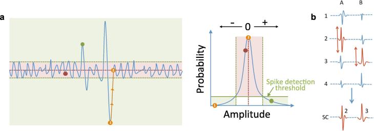
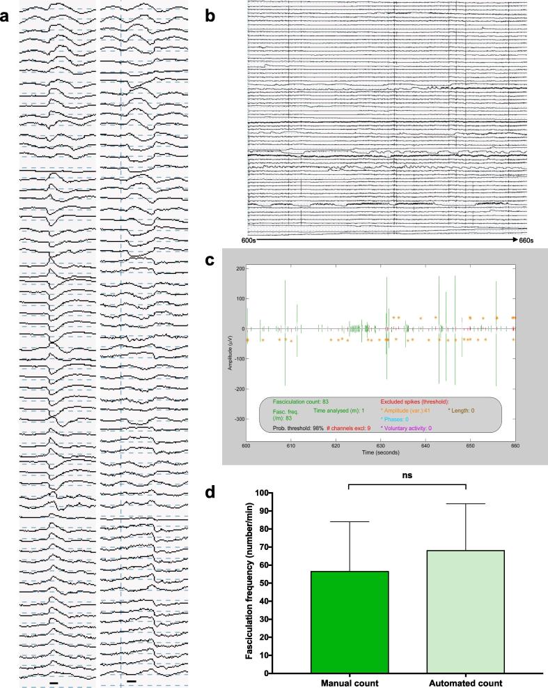
Objectives: Fasciculations are a clinical hallmark of amyotrophic lateral sclerosis (ALS). Compared to concentric needle EMG, high-density surface EMG (HDSEMG) is non-invasive and records fasciculation potentials (FPs) from greater muscle volumes over longer durations. To detect and characterise FPs from vast data sets generated by serial HDSEMG, we developed an automated analytical tool.

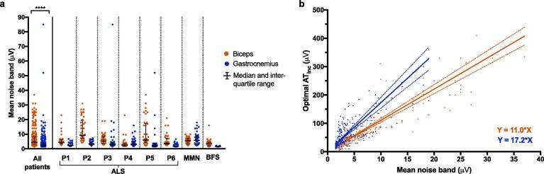
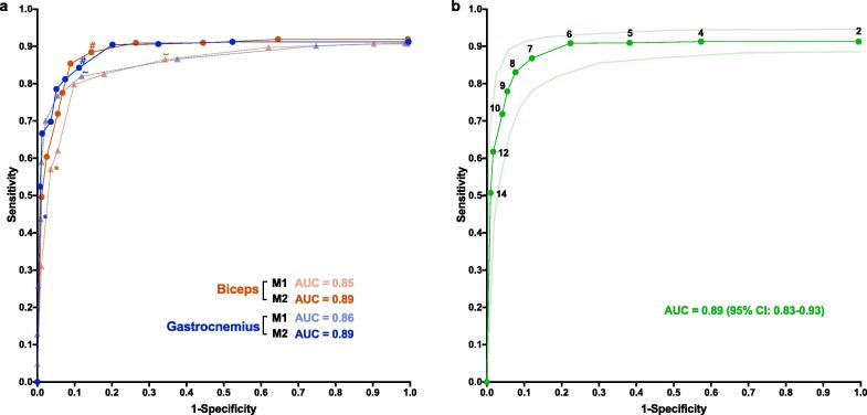
Methods: Six ALS patients and two control patients (one with benign fasciculation syndrome and one with multifocal motor neuropathy) underwent 30-minute HDSEMG from biceps and gastrocnemius monthly. In MATLAB we developed a novel, innovative method to identify FPs amidst fluctuating noise levels. One hundred repeats of 5-fold cross validation estimated the model's predictive ability.

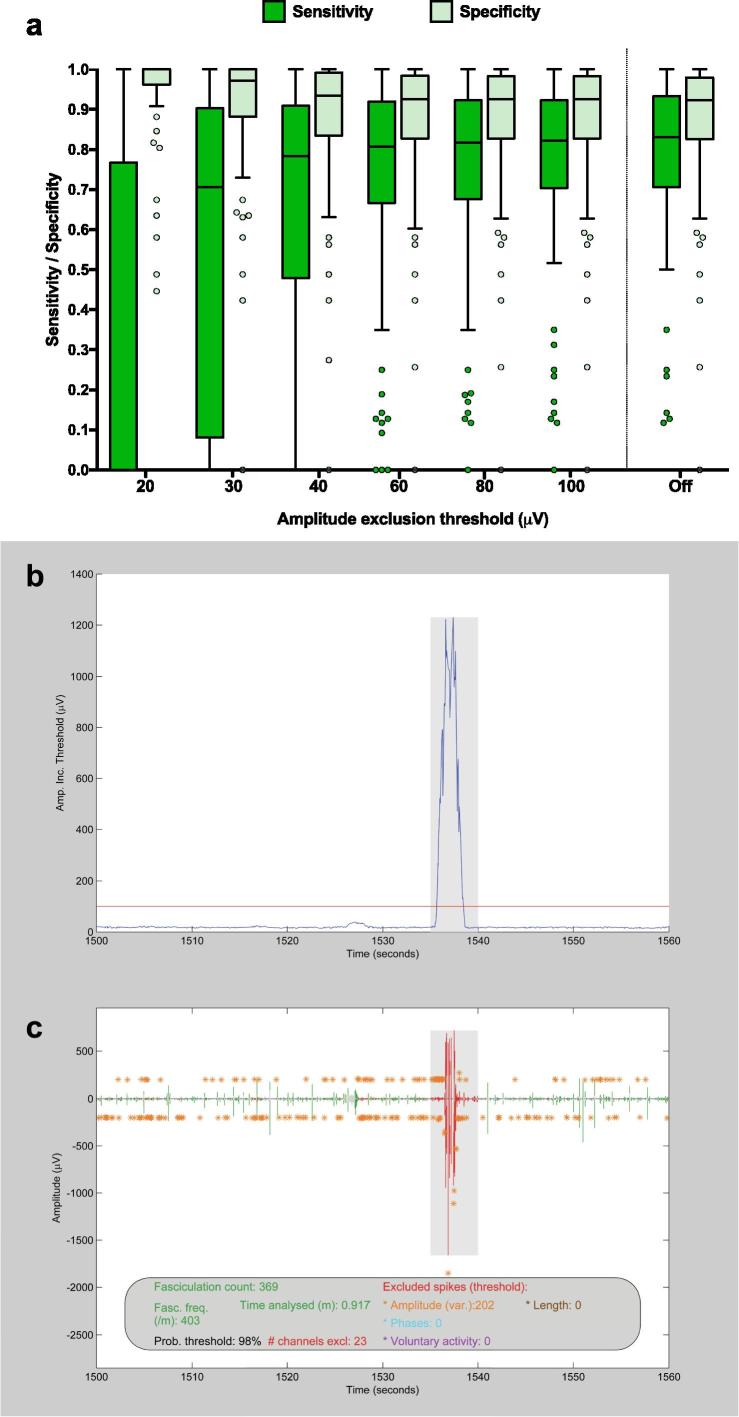
Results: By applying this method, we identified 5,318 FPs from 80 minutes of recordings with a sensitivity of 83.6% (+/- 0.2 SEM), specificity of 91.6% (+/- 0.1 SEM) and classification accuracy of 87.9% (+/- 0.1 SEM). An amplitude exclusion threshold (100 μV) removed excessively noisy data without compromising sensitivity. The resulting automated FP counts were not significantly different to the manual counts (p = 0.394).

Conclusion: We have devised and internally validated an automated method to accurately identify FPs from HDSEMG, a technique we have named Surface Potential Quantification Engine (SPiQE).

Significance: Longitudinal quantification of fasciculations in ALS could provide unique insight into motor neuron health.

Keywords: Amyotrophic lateral sclerosis; Biomarker; Fasciculation; High-density surface EMG.

Fig. 1

Data processing. (a) Probability threshold. The spike detection threshold was based on the probability of a given amplitude occurring in the thirty-minute recording. A spike’s duration was found by tracking the spike to its nearest zero point (orange circles). Adjacent phases (positive-negative transition) were joined and recorded as a single spike. (b) Principle of the super-channel (SC). For spikes A and B, the channel (1–4) with the highest peak-trough amplitude (shown in red) was transferred into the SC. The channel of origin for each spike was stored. (For interpretation of the references to colour in this figure legend, the reader is referred to the web version of this article.).

Fig. 2

Noise level analysis (phase one). (a) Distribution of mean noise bands for biceps and gastrocnemius. Each data point represents one minute of recording. There was a significant difference in noise levels between biceps and gastrocnemius (p < 0.0001, Mann-Whitney test). (b). Relationships between mean noise band and optimal AT_inc. AT_inc was calculated from manual counts using 10 s windows. The best-fit lines were calculated with weighted least-squares regression due to heteroscedasticity of the data. For biceps (red), n was 295 and r² was 0.648. For gastrocnemius (blue), n was 304 and r² was 0.402. (For interpretation of the references to colour in this figure legend, the reader is referred to the web version of this article.).

Fig. 3

Receiver operating characteristic (ROC) curves for FP identification (phase three). (a) Comparison of two analytical models. For each muscle (biceps in red and gastrocnemius in blue), 40 one-minute representative recordings were analysed. Model one (M1, triangle symbols) took the form Y = A₁ and model two (M2, circular symbols) took the form Y = A₂X_, where Y was the optimal AT_inc (μV), X was the mean noise band (μV) and A_1/2 was a positive value. From left-to-right, threshold values for A₁ were 100, 60, 40, 35, 30, 25, 20, 15, 10 and 5, and values for A₂ were 14, 12, 10, 9, 8, 7, 6, 5, 4 and 2. Median sensitivity and specificity are displayed (non-parametric distributions). Area-under-the curve (AUC, 2 s.f.) represents the accuracy of each model for each muscle. * indicates the performance of M1 when A₁ = 40; ∼ indicates performance of M1 when A₁ = 20; # indicates the performance of M2 when A₂ = 7. (b) Pooled results for model two. The results from biceps and gastrocnemius were pooled to produce a total of 80 one-minute recordings. Threshold values for A₂ are displayed. Curves for median sensitivity and specificity are plotted alongside lower and upper limits for 95% confidence interval (CI). AUC represents the accuracy of this model. (For interpretation of the references to colour in this figure legend, the reader is referred to the web version of this article.).

Fig. 4

Data exclusion. (a) Finding the optimal amplitude exclusion threshold (AT_exc). The AT_exc was varied to calculate the sensitivity and specificity for 80 pooled (biceps and gastrocnemius) one-minute recordings. Boxes represent median and inter-quartile range (IQR). Whiskers represent (upper quartile + 1.5 * IQR) and (lower quartile − 1.5 * IQR) according to Tukey’s method. Data points beyond this range are plotted individually. (b) AT_exc example - part 1. One minute of amplitude inclusion thresholds (linearly related to noise levels), showing a burst in noise levels between 1535–1540 s. Amplitude exclusion threshold of 100 μV (red line) applied to exclude shaded region. (c) AT_exc example - part 2. Corresponding one minute of super-channel recording, showing exclusion of noisy period. Fasciculation count (369), time analysed (0.917 m) and fasciculation frequency (403/m) have been automatically adjusted. (For interpretation of the references to colour in this figure legend, the reader is referred to the web version of this article.)

Fig. 5

Application of the analytical pipeline. (a) FPs from raw data. Black bar indicates 5 ms duration. (b) Example raw data. 60 s of raw data from gastrocnemius of ALS patient 3. (c) Example SPiQE output. Super-channel of corresponding 60 s of data in ‘b’ after application of optimal analytical pipeline. (d) Model performance. The optimal model (Y = 8X) has been applied to 80 one-minute recordings and compared with high precision manual counts. Medians and 95% confidence intervals plotted. Wilcoxon signed-rank test confirms no significant difference (p = 0.394).

References

1. Al-Chalabi A., Hardiman O. The epidemiology of ALS: a conspiracy of genes, environment and time. Nat Rev Neurol. 2013;9:617–628. - PubMed
1. Benatar M., Boylan K., Jeromin A., Rutkove S.B., Berry J., Atassi N., Bruijn L. ALS biomarkers for therapy development: State of the field and future directions. Muscle Nerve. 2016;53:169–182. - PMC - PubMed
1. Bensimon G., Lacomblez L., Meininger V. A controlled trial of riluzole in amyotrophic lateral sclerosis. ALS/Riluzole Study Group. N Engl J Med. 1994;330:585–591. - PubMed
1. Brooks B.R., Miller R.G., Swash M., Munsat T.L. El Escorial revisited: revised criteria for the diagnosis of amyotrophic lateral sclerosis. Amyotroph Lateral Scler Other Motor Neuron Disord. 2000;1:293–299. - PubMed
1. Cedarbaum J.M., Stambler N., Malta E., Fuller C., Hilt D., Thurmond B., Nakanishi A. The ALSFRS-R: a revised ALS functional rating scale that incorporates assessments of respiratory function. BDNF ALS Study Group (Phase III) J Neurol Sci. 1999;169:13–21. - PubMed
Publication types