Cascaded Tuning to Amplitude Modulation for Natural Sound Recognition

Abstract

The auditory system converts the physical properties of a sound waveform to neural activities and processes them for recognition. During the process, the tuning to amplitude modulation (AM) is successively transformed by a cascade of brain regions. To test the functional significance of the AM tuning, we conducted single-unit recording in a deep neural network (DNN) trained for natural sound recognition. We calculated the AM representation in the DNN and quantitatively compared it with those reported in previous neurophysiological studies. We found that an auditory-system-like AM tuning emerges in the optimized DNN. Better-recognizing models showed greater similarity to the auditory system. We isolated the factors forming the AM representation in the different brain regions. Because the model was not designed to reproduce any anatomical or physiological properties of the auditory system other than the cascading architecture, the observed similarity suggests that the AM tuning in the auditory system might also be an emergent property for natural sound recognition during evolution and development.SIGNIFICANCE STATEMENT This study suggests that neural tuning to amplitude modulation may be a consequence of the auditory system evolving for natural sound recognition. We modeled the function of the entire auditory system; that is, recognizing sounds from raw waveforms with as few anatomical or physiological assumptions as possible. We analyzed the model using single-unit recording, which enabled a fair comparison with neurophysiological data with as few methodological biases as possible. Interestingly, our results imply that frequency decomposition in the inner ear might not be necessary for processing amplitude modulation. This implication could not have been obtained if we had used a model that assumes frequency decomposition.

Keywords: amplitude modulation; deep neural network; neural tuning; single-unit recording.

Figure 1.

Rich repertoires of AM in natural sounds. a, Examples of sound waveforms (gray) and their amplitude envelopes (black) of natural sounds. Sounds of speech (top) and rain (bottom) are shown. b, Modulation spectra showing the distributions of the AM components of the sounds in a. The modulation spectrum was calculated as the RMS of the filtered envelope with a logarithmically spaced band-pass filter bank. Each modulation spectrum was normalized by its maximum value. The lower and upper peaks in the modulation spectrum of speech (top) probably contain information about the speech content and the speaker, respectively. The modulation spectrum of the rain sound (bottom) appeared different from that of speech.

Figure 2.

DNN architecture. Our DNN consists of a stack of one-dimensional dilated convolutional layers. The figure shows the architecture of the DNN for natural sounds. Each layer contains 128 units and performs dilated convolution followed by a nonlinear activation function. The first layer takes a raw sound waveform as an input and the highest layer is connected to the classification layer, which was excluded from the analysis. The output is the category label assigned to the classification unit with maximum activation. We tested multiple architectures with random filter and dilation lengths in each convolutional layer and selected the DNN that achieved the best classification accuracy on the novel dataset. The filter and dilation lengths in all the layers are shown in Table 1. The numbers of layers and units in each layer were chosen in the pilot experiment.

Figure 3.

Confusion matrices of classification of validation data. There are 18 categories. The labels of the true categories are shown in the ordinates and those of the predicted categories are shown in the abscissas. The value in each cell is calculated as the time frame fractions classified as a particular category among the total number of time frames with the true category. Cells with a high classification rate are in the diagonal of the matrices, indicating high classification accuracy. The classification accuracy was defined as the mean values in the diagonal of the matrix.

Figure 4.

Importance of the deep cascade. Classification accuracy of DNNs with various numbers of layers with random filter and dilation lengths. Models with 1, 3, 5, 7, 9, 11, and 13 layers were tested. We tested 32 (blue circles), 64 (orange triangles), and 128 (green squares) channels. DNNs with 13 layers and 32 or 64 channels were not tested because they were excluded by the pilot study. The deeper the DNN, the higher the classification accuracy appeared to be. The result indicates the importance of the deep cascade.

Figure 5.

Single-unit recording in the DNN. a, Illustrations of single-unit recording in a brain (top) and in a DNN (bottom). In physiological experiments, neural activities are recorded while presenting an AM sound stimulus to the animal. We simulated the method and recorded the unit activities of the DNN while feeding it an AM sound stimulus. b, Examples of AM stimuli with 1, 10, 100, and 1000 Hz AM rates. The carrier was white noise. Temporally magnified plots are shown on the right. c, Examples of responses to the AM stimuli in b in a single unit. A unit in the eighth layer is chosen as an example. d, An example of tMTF (top) and rMTF (bottom) in the same unit as in c. A tMTF and an rMTF are defined as synchrony with the stimulus AM rate and the average activity as functions of AM rate, respectively. The unit exhibited the low-pass type tMTF and the band-pass type rMTF.

Figure 6.

Emergent AM tunings in the DNN. a, Examples of tMTFs (left), and rMTFs (right) in the first, fifth, ninth, and 13^th layers. The layers are sorted vertically from bottom to top. One example of a low-pass (solid green line), a band-pass (dashed red line), and a flat (dash-dotted gray line) MTF is shown for each layer. b, Number of units with the low-pass (solid green lines with circles), band-pass (dashed red lines with crosses), high-pass (dotted black lines with triangles), and flat (dash-dotted gray lines with squares) type tMTFs (left) and rMTFs (right). c, Heat maps of all tMTFs (left) and rMTFs (right) in the first, fifth, ninth, and 13^th layers. The MTFs are normalized by their peak values for better visualization. The units are sorted vertically by their peak AM rates. In some layers, distinct peaks and notches appeared commonly across different units at particular AM rates (observed as vertical lines in tMTFs). We have no clear explanation for these features, but they are probably due to artifacts of discrete convolutional operation.

Figure 7.

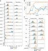
Similar distributions of MTF shapes in the DNN and those in the auditory system. a, Histograms of BMF (filled blue bars) and UCF (hatched orange bars) of temporal (left) and rate (right) coding in each layer. The layers are sorted vertically from bottom to top. b, Number of units with a definable BMF (filled blue circles) and UCF (open orange triangles) of temporal (solid lines) and rate (dashed lines) coding. c, Distributions of BMF (filled blue areas) and UCF (hatched orange areas) of the temporal (left) and rate (right) coding in each region in the auditory system. Regions are sorted vertically from the peripheral region (bottom) to the central region (top). No distribution is drawn where none is reported.

Figure 8.

Similarity to the auditory system throughout the entire cascade revealed by the layer–region pairwise similarity. a, Layer–region pairwise similarities of BMF (top) and UCF (bottom) of temporal (left) and rate (right) coding. The four pairwise similarities were averaged to yield the final layer–region pairwise similarity shown in b. In all of them, the lower, middle, and upper layers appeared to be similar to the peripheral, middle, and central brain regions, respectively, although the similarities are not as smooth or clear as their average. b, Layer–region pairwise similarity of the AM representation in the DNN layers (horizontal axis) and that in the regions in the auditory system (vertical axis). c, Layer–region pairwise similarity normalized by the maximum value of each brain region.

Figure 9.

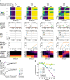
Development of AM representation in the DNN during optimization. a, From top to bottom: heat maps of all tMTFs (left) and rMTFs (right) in the first, fifth, ninth, and 13^th layers (as in Fig. 6c); the number of units with low-pass, band-pass, high-pass, and flat MTFs (as in Fig. 6b); histograms of BMFs and UCFs of temporal (left) and rate (right) coding (as in Fig. 7a); number of units with definable tBMF, tUCF, rBMF, and rUCF (as in Fig. 7b); and layer–region pairwise similarity (as in Fig. 8b). The progress of the optimization and the classification accuracy is shown at the top of each column. Auditory-system-like AM tuning gradually emerged as optimization progressed. b, Classification accuracy (top) and cascade similarity (bottom) as functions of the progress of optimization. The progress of optimization, shown on the horizontal axis, is linearly scaled so that the value is 1 at the end of the optimization. Colored markers indicate the points at which the layerwise similarities were calculated in c. c, Layerwise similarity at four intermediate snapshot instances during optimization. Colors, markers, and lines indicate the progress of optimization as indicated by the legend and in b.

Figure 10.

Evaluation of the similarity of the entire cascade. The cascade similarity was defined as the weighted mean of the pairwise similarity matrix. The weight was designed to be larger near the diagonal line and smaller in the top left and bottom right corners. The layerwise similarity was defined as the mean calculated across brain regions within each layer.

Figure 11.

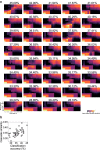
Cascade similarity of DNNs with various architectures correlated with their classification accuracy. a, Heat maps showing the layer–region pairwise similarity sorted in terms of classification accuracy, which is shown at the top of each panel. The top left panel is identical to Figure 8b. Pairwise similarities along a diagonal line appeared larger in DNNs with high classification performance. b, Cascade similarities of DNNs with various architectures plotted against their classification accuracies. A single circle represents a single architecture.

Figure 12.

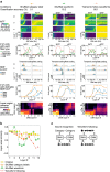
AM representation in DNN with control conditions. a, AM representation in a DNN trained on shuffled category labels (left column), on shuffled waveform (middle column), and optimized for the waveform following task (right column). Colored symbols and lines by the panel titles indicate the types of control condition as in b. Other conventions are the same as in Figure 9a. b, Layerwise similarity in the control experiments. The similarities under the original condition (yellow diamonds and solid line) are also shown. c, Schematic illustration of recognition and waveform following tasks. In both tasks, the DNN operated on a short sound segment. The sound recognition task was to estimate the category of the input sound. The waveform following task was to copy the amplitude value of the last time frame of the input segment.

Figure 13.

Similarity emerges consistently from speech dataset. a, Confusion matrices of the classification of the validation data. There are 39 categories. Other conventions are the same as in Figure 3. b, Layer–region pairwise similarity normalized by the maximum value for each brain region. Other conventions are the same as in Figure 8c c, Classification accuracy (top) and cascade similarity (bottom) as functions of the progress of optimization. d, Layer–region pairwise similarity after and before optimization, that of the DNN trained on shuffled category labels and shuffled waveforms, and that of the waveform-following task. e, Cascade similarities of DNNs with various architectures plotted against their classification accuracies. All results were consistent with those obtained with the nonhuman natural sound.

Figure 14.

Histograms of tMTF sharpness. Layers 3, 5, 7, 9, 11, and 13 are shown as examples. The Q factors in the first and second layers are not calculated because no units in these layers were band-pass shaped. SDs are shown in the top right corners.

Figure 15.

Tuning to acoustic frequency. a, AF tuning in four example units in each layer. Red and blue, respectively, indicate larger and smaller responses than the silent stimulus. White indicates a response equal to silence. Black and gray lines show the AF tuning curves. The thresholds were 0.1 (light gray lines), 0.01 (dark gray lines), and 0.001 (black lines) above the response to silence. Generally, the responses appeared monotonic along the stimulus amplitude, but some units in the upper layers exhibited a nonmonotonic response along the stimulus amplitude. The AF tuning curves did not show clear single troughs. b, AF tuning curves in all the units in each layer. The curves are shown for thresholds of 0.001 (left), 0.01 (middle), and 0.1 (right) above the response to silence. The units in each layer are sorted by the trough frequency of the tuning curves. Troughs in the AF tuning curves in the middle layers appear to cover a wide AF range, but not in the lower and higher layers.

References

1. Aytar Y, Vondrick C, Torralba A (2016) SoundNet: learning sound representations from unlabeled video. Adv Neural Inf Process Syst 29:892–900.
1. Bacon SP, Grantham DW (1989) Modulation masking: Effects of modulation frequency, depth, and phase. J Acoust Soc Am 85:2575–2580. 10.1121/1.397751 - DOI - PubMed
1. Bartlett EL, Wang X (2007) Neural representations of temporally modulated signals in the auditory thalamus of awake primates. J Neurophysiol 97:1005–1017. 10.1152/jn.00593.2006 - DOI - PubMed
1. Batra R. (2006) Responses of neurons in the ventral nucleus of the lateral lemniscus to sinusoidally amplitude modulated tones. J Neurophysiol 96:2388–2398. 10.1152/jn.00442.2006 - DOI - PubMed
1. Batra R, Kuwada S, Stanford TR (1989) Temporal coding of envelopes and their interaural delays in the inferior colliculus of the unanesthetized rabbit. J Neurophysiol 61:257–268. 10.1152/jn.1989.61.2.257 - DOI - PubMed
Publication types
LinkOut - more resources