An algorithm for learning shape and appearance models without annotations

Abstract

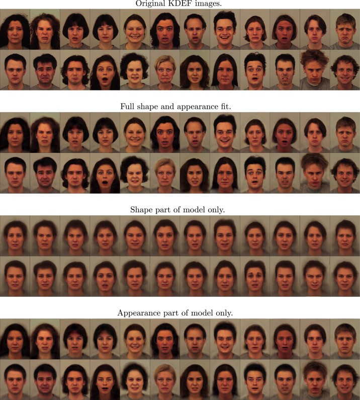
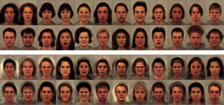
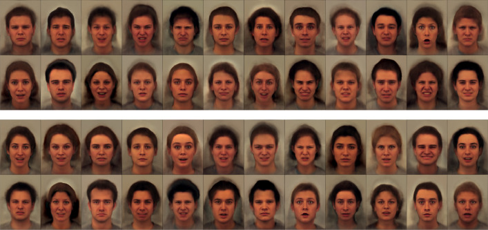
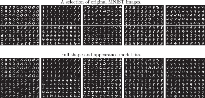
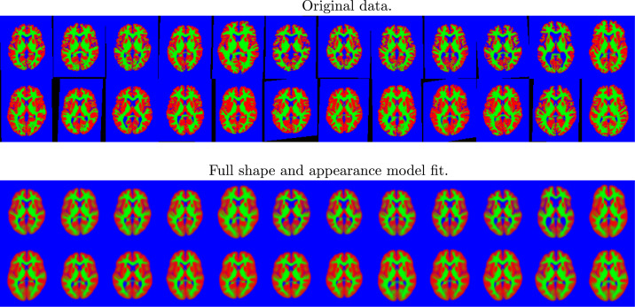
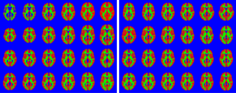
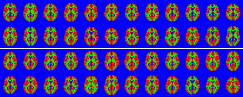
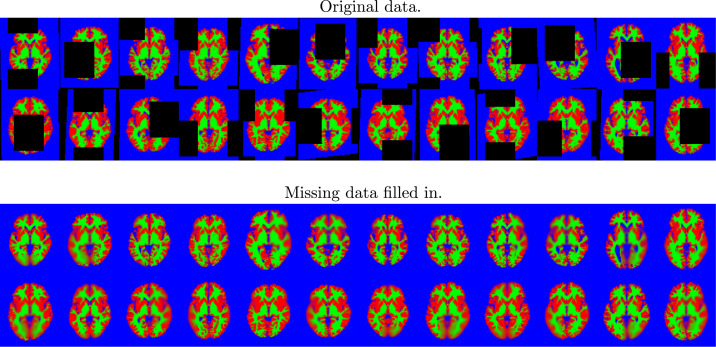
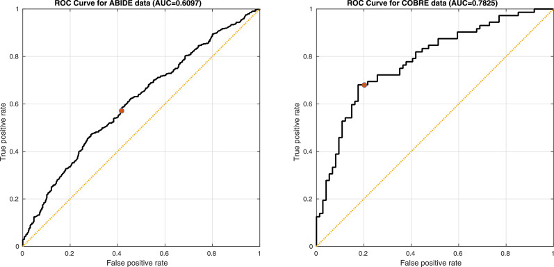
This paper presents a framework for automatically learning shape and appearance models for medical (and certain other) images. The algorithm was developed with the aim of eventually enabling distributed privacy-preserving analysis of brain image data, such that shared information (shape and appearance basis functions) may be passed across sites, whereas latent variables that encode individual images remain secure within each site. These latent variables are proposed as features for privacy-preserving data mining applications. The approach is demonstrated qualitatively on the KDEF dataset of 2D face images, showing that it can align images that traditionally require shape and appearance models trained using manually annotated data (manually defined landmarks etc.). It is applied to the MNIST dataset of handwritten digits to show its potential for machine learning applications, particularly when training data is limited. The model is able to handle "missing data", which allows it to be cross-validated according to how well it can predict left-out voxels. The suitability of the derived features for classifying individuals into patient groups was assessed by applying it to a dataset of over 1900 segmented T1-weighted MR images, which included images from the COBRE and ABIDE datasets.

Keywords: Appearance model; Diffeomorphisms; Geodesic shooting; Latent variables; Machine learning; Shape model.

Graphical abstract

Fig. 1

A graphical representation of the model (showing only the 1st strategy). Gray circles indicate observed data, whereas white circles indicate variables that are either estimated (W^v, W^a, μ and z) or marginalised out (A). The plate indicates replication over all images.

Algorithm 1

Shape and appearance model.

Algorithm 2

Computing gradients and Hessians for mean.

Algorithm 3

Likelihood derivatives for Gaussian noise model.

Algorithm 4

Geodesic shooting via Euler integration.

Algorithm 5

Computing gradients and Hessians for appearance.

Algorithm 6

Computing gradients and Hessians for shape.

Algorithm 7

Updating latent variables.

Algorithm 8

Orthogonalising the variables.

Fig. 2

Shape and appearance fit shown for a randomly selected sample of the KDEF face images. (For interpretation of the references to colour in this figure legend, the reader is referred to the web version of this article.)

Fig. 3

Fits using a simple 64-mode principal component analysis model are shown above (cf. Fig. 2), and random faces generated from the same PCA model are shown below (cf. Fig. 4). (For interpretation of the references to colour in this figure legend, the reader is referred to the web version of this article.)

Fig. 4

Random faces generated from the shape and appearance model. The lower set of faces were generated with the same latent variables as those shown in the upper set, except the values were multiplied by −1 and thus show a sort of “opposite” face. For example, if a face in the top set has a wide open mouth, then the mouth should be tightly closed in the corresponding image of the bottom set. (For interpretation of the references to colour in this figure legend, the reader is referred to the web version of this article.)

Fig. 5

An example of simple linear additions and subtractions applied to the latent variables. The first three columns show the full shape and appearance model fits to various faces. Images in the right hand column were generated by making linear combinations of the latent variables that encode the images in the first three columns, and then reconstructing from these linear combinations. (For interpretation of the references to colour in this figure legend, the reader is referred to the web version of this article.)

Fig. 6

A random selection of digits from the first 10,000 MNIST training images, along with the model fit. In general, good alignment is achieved.

Fig. 7

Left: Test errors from training the method using different sized subsets of the MNIST data (the error rate from random guessing would be 90%). Right: All the MNIST digits the method failed to correctly identify (after training with the full 60,000) are shown above. These are followed by the model fits for the true digit, and then the model fits for the incorrect guess (i.e., the one with the most model evidence). (For interpretation of the references to colour in this figure legend, the reader is referred to the web version of this article.)

Fig. 8

Illustration of the non-Gaussian distributions of the latent variables for some of the MNIST digits. Plots of selected latent variables are shown above, with the corresponding modes of variation shown below. Gaussian mixture models are likely to provide better models of variability than the current assumption of a single Gaussian distribution.

Fig. 9

A random selection of the 2D brain image data, showing grey matter (red), white matter (green) and other (blue). Black regions indicate missing data. Below these is the model fit to the images. (For interpretation of the references to colour in this figure legend, the reader is referred to the web version of this article.)

Fig. 10

First eight (out of a total of 100) modes of variability found from the 2D brain image dataset, shown at −5, −3, −1, +1, +3 & +5 standard deviations. Note that these modes encode some topological changes, in addition to changes in shape. (For interpretation of the references to colour in this figure legend, the reader is referred to the web version of this article.)

Fig. 11

Randomly generated slice through brain images. These images were constructed by using randomly assigned latent variables. Note that the top set of images uses the same random variables as the bottom set, except they are multiplied by $-1$. This means that one set is a sort of “opposite” of the other. For example, if a brain in the upper set has large ventricles, then the corresponding brain in the lower set will have small ventricles. (For interpretation of the references to colour in this figure legend, the reader is referred to the web version of this article.)

Fig. 12

A random selection of the 2D brain image data showing the location of missing data. The attempt to fill in the missing information is shown below. These may be compared against the original images shown in Fig. 9. (For interpretation of the references to colour in this figure legend, the reader is referred to the web version of this article.)

Fig. 13

Cross-validation accuracy measures based on predicting the left-out patches of the images using different model configurations. The blue dots show the mean value for each of the 1913 images, whereas the horizontal bars show the mean values overall. The plot on the left shows mean log-likelihoods over the pixels in each patch, wheres the plot on the right shows the log-likelihoods after subtracting the mean – over model configurations – for each patch.

Fig. 14

Cross-validation accuracy measures based on predicting the left-out patches of the images using different hyper-parameter settings. The blue dots show the mean value for each of the 1913 images, whereas the horizontal bars show the mean values overall. Accuracy measures are mean log-likelihoods (over voxels), after adjustment.

Fig. 15

An illustration of the mean images from the 2D and 3D experiments (after Softmax). Left: The mean image from the 2D experiments (c.f. Figs. 9 and 10). Right: Slice 40 of the mean image from the 3D experiment. (For interpretation of the references to colour in this figure legend, the reader is referred to the web version of this article.)

Fig. 16

ROC curves from five-fold cross-validation accuracies from the ABIDE and COBRE data. Red dots show the point on the curve where the classification gives probabilities of 0.5.

Fig. 17

Overlap measures from the two registration approaches. Diagonal lines are spaced two standard deviations apart. Circled points indicate outliers of more than two standard deviations.

Fig. 18

Mid-sagittal slice through the basis functions. The mean (μ) and four appearance basis functions (W^a) are shown above, while the divergences of the first 10 shape basis functions (W^v) are shown below.

References

1. Adams D., Rohlf F., Slice D. Geometric morphometrics: ten years of progress following the ‘revolution’. Ital. J. Zool. 2004;71(1):5–16.
2. Adams, D., Rohlf, F., Slice, D., 2004. Geometric morphometrics: Ten years of progress following the ‘revolution’. Italian Journal of Zoology 71, 5–16.
1. Allassonnière S., Amit Y., Trouve A. Towards a coherent statistical framework for dense deformable template estimation. J. R. Stat. Soc. Ser. B (Stat. Methodol.) 2007;69(1):3–29.
2. Allassonnière, S., Amit, Y., Trouve, A., 2007. Towards a coherent statistical framework for dense deformable template estimation. Journal of the Royal Statistical Society: Series B (Statistical Methodology) 69, 3–29.
1. Allassonnière S., Durrleman S., Kuhn E. Bayesian mixed effect atlas estimation with a diffeomorphic deformation model. SIAM J. Imaging Sci. 2015;8(3):1367–1395.
2. Allassonnière, S., Durrleman, S., Kuhn, E., 2015. Bayesian mixed effect atlas estimation with a diffeomorphic deformation model. SIAM Journal on Imaging Sciences 8, 1367–1395.
1. Ashburner J. A fast diffeomorphic image registration algorithm. Neuroimage. 2007;38(1):95–113. - PubMed
2. Ashburner, J., 2007. A fast diffeomorphic image registration algorithm. Neuroimage 38, 95–113. - PubMed
1. Ashburner J., Friston K. Unified segmentation. Neuroimage. 2005;26(3):839–851. - PubMed
2. Ashburner, J., Friston, K., 2005. Unified segmentation. Neuroimage 26, 839–851. - PubMed
Publication types