Host diet and evolutionary history explain different aspects of gut microbiome diversity among vertebrate clades

Abstract

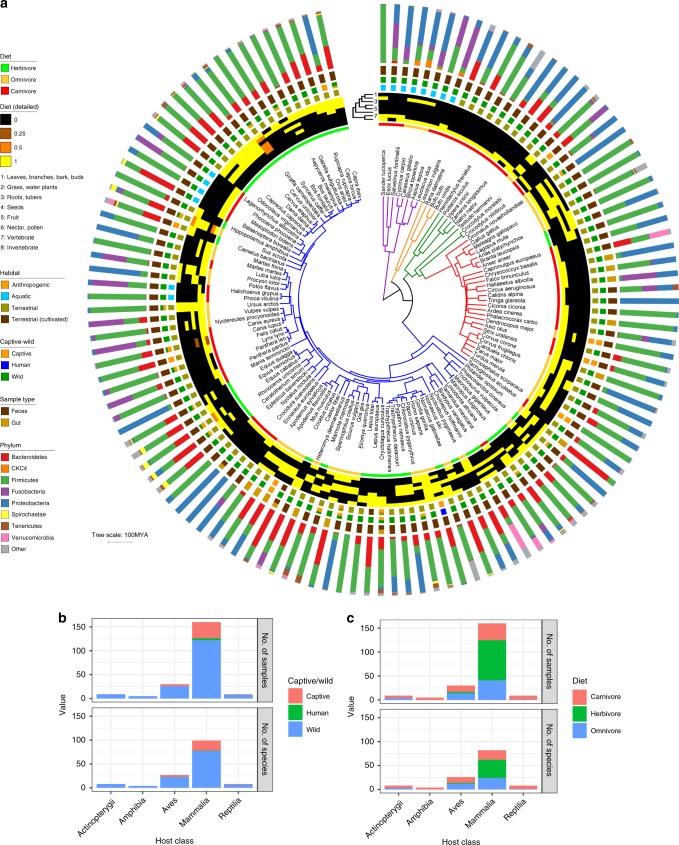
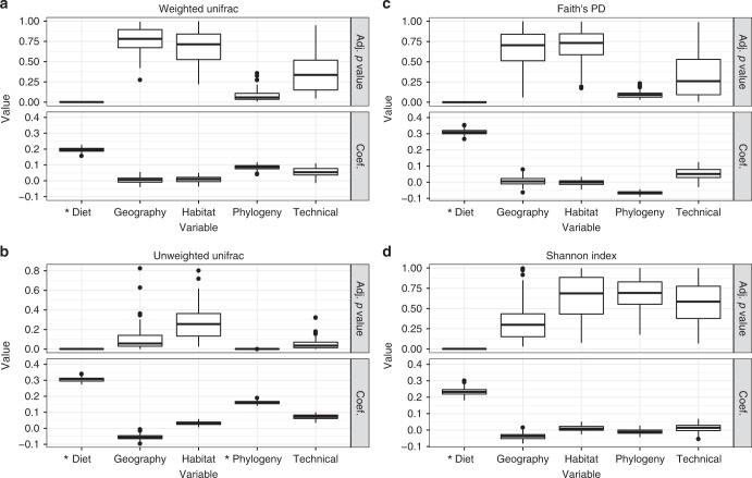
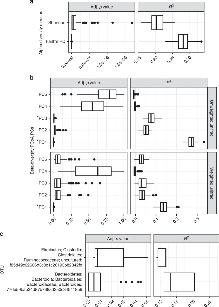
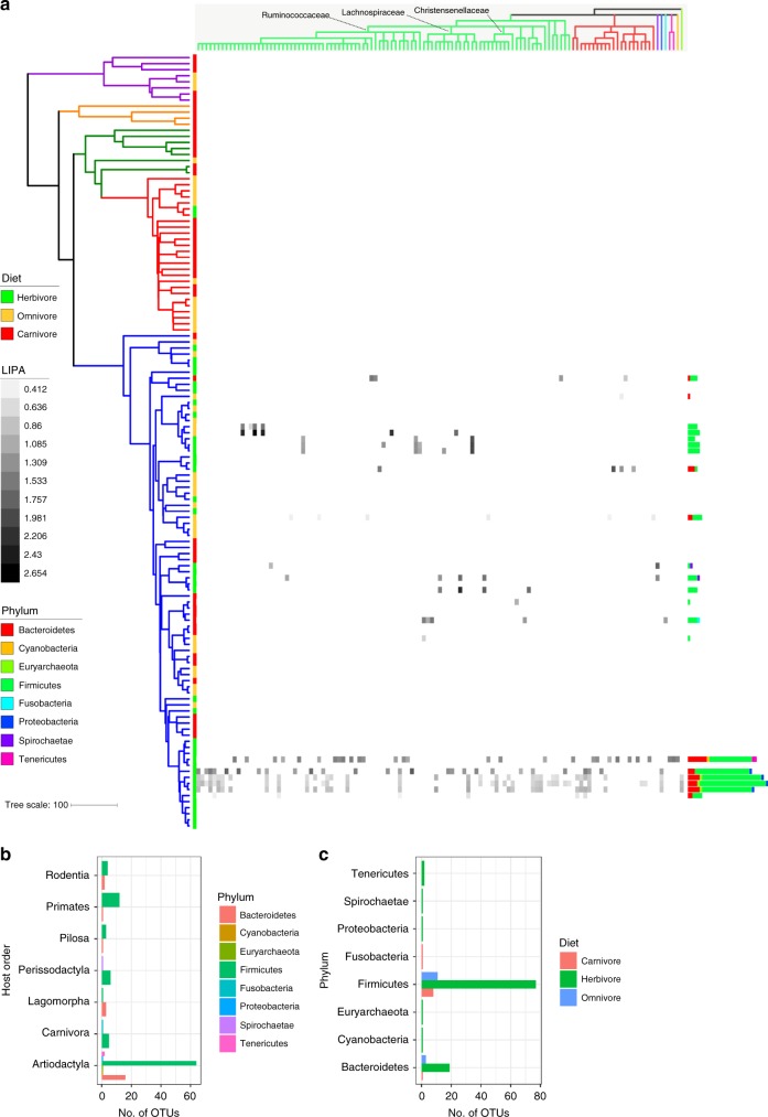
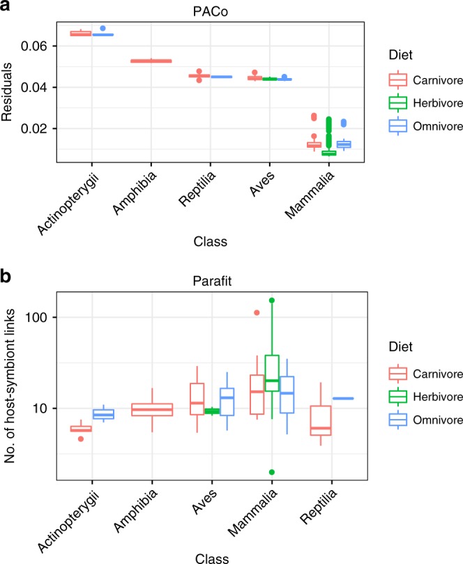
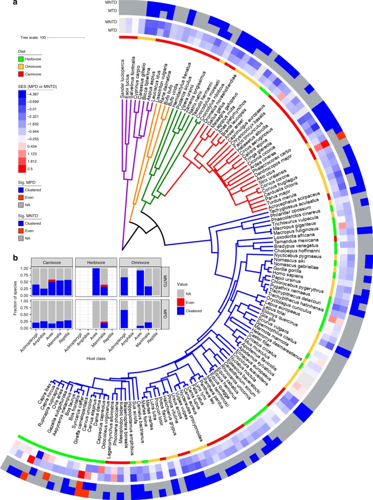
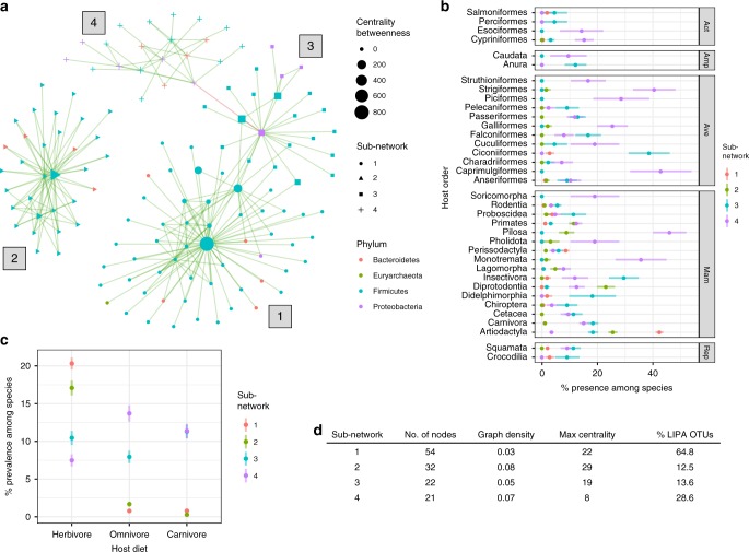
Multiple factors modulate microbial community assembly in the vertebrate gut, though studies disagree as to their relative contribution. One cause may be a reliance on captive animals, which can have very different gut microbiomes compared to their wild counterparts. To resolve this disagreement, we analyze a new, large, and highly diverse animal distal gut 16 S rRNA microbiome dataset, which comprises 80% wild animals and includes members of Mammalia, Aves, Reptilia, Amphibia, and Actinopterygii. We decouple the effects of host evolutionary history and diet on gut microbiome diversity and show that each factor modulates different aspects of diversity. Moreover, we resolve particular microbial taxa associated with host phylogeny or diet and show that Mammalia have a stronger signal of cophylogeny. Finally, we find that environmental filtering and microbe-microbe interactions differ among host clades. These findings provide a robust assessment of the processes driving microbial community assembly in the vertebrate intestine.

Fig. 1

Phylum-level grouping of microbiome diversity by host phylogeny and host metadata. a The dated host phylogeny was obtained from http://timetree.org, with branches colored by host class (purple = Actinopterygii; orange = Amphibia; green = Reptilia; red = Aves; blue = Mammalia). From inner to outer, the data mapped onto the tree is host diet (general), host diet (detailed breakdown), host habitat, host captive/wild status, the microbiome sample type, and the relative abundances of microbial phyla in each host. Relative abundances are an estimated average generated via subsampling operational taxonomic units from all samples for each host species (subsampling to 5000 for each host species). Note that “Diet (detailed)” information varies among some individuals, and the values shown are averages of the binary yes/no values (no = 0; yes = 1) for each individual. For example, the Giraffa camelopardalis samples are from two captive and two wild individuals, so the dietary information somewhat differs, resulting in intermediate values (orange). b, c show the number of samples or host species per class colored by captive/wild status or diet, respectively. Source data are provided as a Source Data file

Fig. 2

Host phylogeny and diet significantly explain the aspects of microbiome diversity. The plots show the BH-adjusted p values (Adj. p value) and partial regression coefficients (Coef.) for multiple regression on matrix (MRM) tests used to determine how much alpha- or beta-diversity variance was explained by host diet, geographic location, habitat, phylogeny, and technical parameters (see “Methods”). The boxplots show the distribution of values obtained when running MRM on each of the 100 random dataset subsets, with each subsample comprising just one sample per species. The boxplots show the MRM rho coefficient and p value for each subsample. See “Methods” for a description of how each distance matrix for the MRM models was generated. Asterisk denotes significance (Adj. p < 0.05 for ≥95% of dataset subsets; see “Methods”). Box centerlines, edges, whiskers, and points signify the median, interquartile range (IQR), 1.5× IQR, and >1.5× IQR, respectively. Source data are provided as a Source Data file

Fig. 3

After accounting for host phylogeny, diet significantly explained alpha- and beta-diversity components but could only explain the prevalence of two operational taxonomic units (OTUs). The boxplots are distributions of phylogenetic generalized least squares R² and Adj. p for 100 random subsamples of the datasets (one per species for each subsample). a Both alpha-diversity measures were found to be significant. b Some principal component (PC) analysis PCs were significantly explained by diet (asterisk denotes Adj. p < 0.05). The percentage of variance explained for each unweighted Unifrac PC is 18.1, 6.9, 4.2, 3.6, and 2.1 and each weighted Unifrac PC is 27.2, 10.6, 9.6, 6.4, 6.0, and 5.5. c Only two OTUs were found to be significant. Box centerlines, edges, whiskers, and points signify the median, interquartile range (IQR), 1.5× IQR, and >1.5× IQR, respectively. Source data are provided as a Source Data file

Fig. 4

Many operational taxonomic units (OTUs) display a local phylogenetic signal in specific host clades after accounting for diet. a The phylogeny is the same as shown in Fig. 1. The heatmap depicts local indicator of phylogenetic association (LIPA) values for each OTU–host association, with higher values indicating a stronger phylogenetic signal of OTU presence (with diet regressed-out). White boxes in the heatmap indicate non-significant LIPA indices. The dendrogram on the top of the heatmap is a cladogram based on the SILVA-derived taxonomy for each OTU (see Supplementary Fig. 18 for the full taxonomy). The dendrogram is colored by phylum. The bar plots in b and c show the number of OTUs with a significant LIPA index per host (OTUs are colored by phylum; the number of OTUs per host ranges from 1 to 34). b The bar plots summarize the number of significant OTUs per host order and diet. The bar plots in c are the same as b except the data are grouped by OTU phylum. Source data are provided as a Source Data file

Fig. 5

Procrustean approach to cophylogeny (PACo) and Parafit show a stronger cophylogeny signal for Mammalia versus non-mammals. a Boxplots of PACo residuals between hosts and operational taxonomic units (smaller residuals means a stronger cophylogeny signal), with residuals grouped by host class and diet. b Boxplots of significant host–symbiont links as determined by Parafit analysis, with links grouped by host class and diet. For both PACo and Parafit, 1000 permutations were performed on each of the 100 dataset subsets. Box centerlines, edges, whiskers, and points signify the median, interquartile range (IQR), 1.5× IQR, and >1.5× IQR, respectively. Source data are provided as a Source Data file

Fig. 6

Microbial communities are generally phylogenetically clustered versus evenly distributed. a The phylogeny is the same as shown in Fig. 1. From inner to outer, the data mapped onto the tree is host diet, mean standardized effect sizes for mean phylogenetic distance (MPD) and mean nearest taxon distance (MNTD), and samples with significant phylogenetic clustering or evenness based on MPD or MNTD. The animal species possessing microbial communities that were phylogenetically evenly distributed were the long-eared owl (Asio otus), fallow deer (Dama dama), red deer (Cervus elaphus), cattle (Bos taurus), and sheep (Ovis aries). b The bar charts depict the fraction of host species for each host class/diet where microbial taxa are more phylogenetically clustered (clustered) or evenly distributed (even) than expected from the null model or those that did not deviate from the null model (NA). Source data are provided as a Source Data file

Fig. 7

Co-occurrence analysis revealed four sub-networks of co-occurring operational taxonomic units (OTUs) that differ in taxonomic composition, network structure, and distribution across host taxonomic orders. a The network is a presence–absence co-occurrence network, with only significant edges shown (see “Methods”). Sub-networks are represented by differing node shapes and labels next to each sub-network. “Centrality betweenness” is a measure of how often the shortest path between two nodes transverses through the focal node. b The distribution of community presence among samples from each species (percentage of samples per species) shown for each host taxonomic order, with points representing the mean and line ranges representing +/− the standard error of the mean. The plots are faceted by host taxonomic class (Act = Actinopterygii, Amp = Amphibia, Ave = Aves, Mam = Mammalia, Rep = Reptilia). c Similar to b but grouped by host diet. d A table of sub-network statistics, with “Graph density” defined as “number of edges/total possible edges,” “Max centrality” defined as the max number of shortest paths between any two nodes that cross the focal node, and “% LIPA OTUs” defined as the percentage of OTUs with significant local phylogenetic signal (Fig. 4). Source data are provided as a Source Data file

References

1. Suzuki TA. Links between natural variation in the microbiome and host fitness in wild mammals. Integr. Comp. Biol. 2017;57:756–769. doi: 10.1093/icb/icx104. - DOI - PubMed
1. McFall-Ngai M, et al. Animals in a bacterial world, a new imperative for the life sciences. Proc. Natl. Acad. Sci. USA. 2013;110:3229–3236. doi: 10.1073/pnas.1218525110. - DOI - PMC - PubMed
1. Rosenberg E, Zilber-Rosenberg I. The hologenome concept of evolution after 10 years. Microbiome. 2018;6:78. doi: 10.1186/s40168-018-0457-9. - DOI - PMC - PubMed
1. Bahrndorff S, Alemu T, Alemneh T, Lund Nielsen J. The microbiome of animals: implications for conservation biology. Int. J. Genomics Proteomics. 2016;2016:5304028. - PMC - PubMed
1. Ley RE, et al. Evolution of mammals and their gut microbes. Science. 2008;320:1647–1651. doi: 10.1126/science.1155725. - DOI - PMC - PubMed
Publication types