Multifractal Desynchronization of the Cardiac Excitable Cell Network During Atrial Fibrillation. II. Modeling

Abstract

In a companion paper (I. Multifractal analysis of clinical data), we used a wavelet-based multiscale analysis to reveal and quantify the multifractal intermittent nature of the cardiac impulse energy in the low frequency range ≲ 2Hz during atrial fibrillation (AF). It demarcated two distinct areas within the coronary sinus (CS) with regionally stable multifractal spectra likely corresponding to different anatomical substrates. The electrical activity also showed no sign of the kind of temporal correlations typical of cascading processes across scales, thereby indicating that the multifractal scaling is carried by variations in the large amplitude oscillations of the recorded bipolar electric potential. In the present study, to account for these observations, we explore the role of the kinetics of gap junction channels (GJCs), in dynamically creating a new kind of imbalance between depolarizing and repolarizing currents. We propose a one-dimensional (1D) spatial model of a denervated myocardium, where the coupling of cardiac cells fails to synchronize the network of cardiac cells because of abnormal transjunctional capacitive charging of GJCs. We show that this non-ohmic nonlinear conduction 1D modeling accounts quantitatively well for the "multifractal random noise" dynamics of the electrical activity experimentally recorded in the left atrial posterior wall area. We further demonstrate that the multifractal properties of the numerical impulse energy are robust to changes in the model parameters.

Keywords: atrial fibrillation; excitable cell network; intermittent dynamics; kinetics of gap junction channel; modeling; multifractal analysis.

Figure 1

(A) Microscopic view of cardiac muscle cells (longitudinal section) stained with hematoxylin (nuclei) and eosin (cytoplasm). The myocardial cells can be recognized by their elongated aspect (50–100 μm long, with sections ~ 10μm), a longitudinal striated organization, multiple branchings and connections at their extremities via intercalated disks (IDs). (B) Schematic GJCs at the onset of depolarization. Depolarizing (resp. polarized) cells are stained in red (resp. blue). Surface charges are depicted with ± symbols, on the inner and outer side of the depolarizing (gray) and polarized (black) membranes and on the dysfunctional GJCs (red) with capacitive charge loading Q_g such that 〈Q_g 〉 = ∫ ρ_g dx. Voltage-gated channel ionic flows are marked with green vertical arrows. Normal GJCs: red resistor symbol, dysfunctional GJCs: gray capacitor symbol. Total currents I (blue horizontal arrow) circulate in opposite directions inside and outside the cell, splitting into the normally flowing ohmic current I_Ω (red), and residual closed GJCs current I_g (dashed red) building up charge. Typical membrane and intercalated disk dimensions are l_m ≈ l_g ∽ 5 nm.

Figure 2

Numerically simulated pseudo bipolar potential. (A) 6 s time-series Δ_b Φ (Equation 12) are generated at positions x (in δx = 0.3 mm units) = 8, 18, 75 and 134 (from top to bottom) with our model defined in Equations (6)–(8) with parameter values defined in Simul #2 (Table 1), L = 150 (in δx = 0.3 mm units). (B) Corresponding Fourier transform power spectra. No attempt was made to reproduce the high and low pass filtering used in real bipolar catheter acquisitions. The natural point source frequency at the boundary is ∽ α γ ≈ 5 Hz. Rarefaction of pulses occurs as one moves away from the source which is a hint at some randomly back-scattered pulses that collide and annihilate up-following pulses without reexciting new pulses.

Figure 3

Wavelet transform of local impulse energy time-series. (A) A 100 s portion of E(t) recorded at the electrode Pt3 (Companion paper I Attuel et al., 2017). (B) Time-scale WT representation of E(t) with the third-order analyzing wavelet g⁽³⁾ (Equation 16). The modulus of the WT is coded, independently at each scale a, using 256 colors from black ($|T_{g^{(3)}}(t,a)|=0$) to red (${max}_t|T_{g^{(3)}}(t,a)|$). (C) WT skeleton defined by the maxima lines of a 10 s portion of E(t). The scale a = αΔt/δt, where α is an analyzing wavelet dependent constant (α = 8.6 10⁻² for g⁽³⁾ with the lastwave software), and δt = 0.4 ms. (A′–C′) same as (A–C) for a numerical time series E(x, t) generated at position x = 75 (in δx = 0.3 mm units) with our model defined in Equations (6)–(8) with the set of parameter values used in Simul #2 (Table 1), and a total system length L = 150 (in δx = 0.3 mm units). In (B′) the white horizontal dashed-dotted lines delimit the range of time scales (2^8.5 ≤ a ≤ 2^13.5) used to perform linear regression fit estimates of the τ(q) and D(h) multifractal spectra.

Figure 4

Multifractal analysis of local impulse energy time-series E(x, t) generated with our model defined in Equations (6)–(8) with the parameter values defined in Simul #2 (Table 1), L = 150 (in δx = 0.3 mm units). (A) log₂Z(q, a) vs. log₂a (Equation 17). (B) h(q, a)/ln 2 vs log₂a (Equation 19). (C) D(q, a)/ln 2 vs. log₂a (Equation 20). The computation were performed with the WTMM method (Paper I, Methods of Analysis Attuel et al., 2017) for different values from q = −1 to 5 with the analyzing wavelet g⁽³⁾ (Equation 16). The vertical dashed lines delimit the range of scales (2^8.5 ≤ a ≤ 2^13.5) used for the linear regression estimate of τ(q), h(q) and D(q) in Figure 5. The symbols correspond to the time-series E(x, t) computed at the spatial positions x = 8 (◦), 18 (□), 75 (▽) and 134 (△) (in δx = 0.3 mm units).

Figure 5

Multifractal spectra of local impulse energy time-series E(x, t) generated with our model defined in Equations (6)–(8) with the set of parameter values defined in Simul #2 (Table 1), L = 150 (in δx = 0.3 mm units). (A) τ(q) vs. q estimated by linear regression fit of log₂Z(q, a) vs. log₂a (Figure 4A). (B) D(h) vs. h obtained from linear regression fits of h(q, a) (Figure 4B) and D(q, a) (Figure 4C) vs. log₂a. The symbols have the same meaning as in Figure 4. The curves correspond to quadratic spectra Equations (23) and (24) with parameters [c₀, c₁, c₂] reported in Table 2 for time-series E(x, t) computed at the spatial positions x = 8 (◦), 18 (□), 75 (▽) and 134 (△) (in δx = 0.3 mm units). For comparison are reported the spectra previously obtained for the experimental time-series recorded at the electrodes Pt3 (blue ▼) and Pt5 (green ▼) in the left atrial posterior wall (Companion paper I Attuel et al., 2017).

Figure 6

Magnitude cumulant analysis of local impulse energy time-series E(x, t) generated with our model defined in Equations (6)–(8) with the set of parameter values defined in Simul #2 (Table 1), L = 150 (in δx = 0.3 mm units). (A) C₁(a)/ln2 vs. log₂a. (B) C₂(a)/ln2 vs. log₂a. (C) C₃(a)/ln2 vs. log₂a. The computation of the C_n(a) (Equation 21) was performed with the third-order analyzing wavelet g⁽³⁾ (Equation 16). The vertical dashed lines delimit the range of scales (2^8.5 ≤ a ≤ 2^13.5) used for the linear regression estimate of coefficients $c_1^{*}$, $c_2^{*}$ and $c_3^{*}$ of τ(q) (Equation 22) reported in Table 1. The symbols have the same meaning as in Figures 4, 5.

Figure 7

Multifractal spectra of local impulse energy time-series E(x, t) generated with our model defined in Equations (6)–(8) with the sets of parameter values defined in Table 1. (A) τ(q) vs. q. (B) D(h) vs. h. These spectra were computed at the same relative spatial position x = L/2 for different lengths L = 30 (Simul #4, ◦, ··· ), 90 (Simul #3, □, - - - - - - 150(Simul#2, ▽, _____), and 210 (Simul #1, △, ) (in δx = 0.3 mm units). The curves correspond to quadratic spectra (Equations 23 and 24) with parameters [c₀, c₁, c₂] reported in Table 3. For comparison are reported the spectra previously obtained from the experimental time-series recorded at the electrodes Pt3 (blue ▼) and Pt5 (green ▼) in the left atrial posterior wall (Companion paper I Attuel et al., 2017).

Figure 8

Multifractal spectra of local impulse energy time-series E(x, t) generated with our model defined in Equations (6)–(8) with the sets of parameter values defined in Simul #6 (Table 1) and L = 150 (in δx = 0.3 mm units). (A) τ(q) vs. q. (B) D(h) vs. h. The spectra were computed at the same relative spatial position x = L/2 = 75 for different conductivities of the fiber: Simul #2 (▽, _____), Simul #6 (+, - - - - -) and Simul #7 (^*, ··· ). The curves correspond to quadratic spectra (Equations 23 and 24) with parameters [c₀, c₁, c₂] reported in Table 4.

Figure 9

Multifractal spectra of local impulse energy time-series E(x, t) generated with our model defined in Equations (6)–(8) with the set of parameter values defined in Simul #5 (Table 1) and L = 150 (in δx = 0.3 mm units). (A) τ(q) vs. q. (B) D(h) vs. h. The spectra were computed with the WTMM method with the third-order analyzing wavelet g⁽³⁾ (Equation 16). 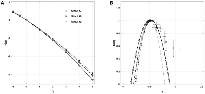The symbols correspond to the spatial positions x = 8 (•, ··· ), 18 (■, - - - - -), 75 (▼, ___________), and 139 (▲, ) (in δx = 0.3 mm units). The curves correspond to quadratic spectra (Equations 23 and 24) with parameters [c₀, c₁, c₂] reported in Table 5. For comparison are reported in open symbols (◦, □, ▽ △), the corresponding spectra previously obtained with the set of parameter values defined in Simul #2 (Table 1) and L = 150 in Figure 5.

Figure 10

Two-point magnitude analysis of local impulse energy time-series E(x, t) generated with our model defined in Equations (6)–(8) with the sets of parameter values defined in Simul #2 (Table 1), L = 150 (in δx = 0.3 mm units). Two-point correlation function C(a, Δt)/C(a, 0) vs. ln (Δt) (Equation 25) computed with the third-order analyzing wavelet g⁽³⁾ (Equation 16). The two curves correspond to scales a = 2⁹ (black) and 2¹⁰ (gray) within the scaling range. The different panels correspond to different spatial positions x = 8 (A), 18 (B), 75 (C), and 134 (D) (in δx = 0.3 mm units).

References

-
- Arneodo A., Audit B., Decoster N., Muzy J.-F., Vaillant C. (2002). A wavelet based multifractal formalism: application to DNA sequences, satellite images of the cloud structure and stock market data, in The Science of Disasters: Climate Disruptions, Heart Attacks, and Market Crashes, eds Bunde A., Kropp J., Schellnhuber H. J. (Berlin: Springer Verlag; ), 26–102.
- Arneodo A., Audit B., Kestener P., Roux S. G. (2008). Wavelet-based multifractal analysis. Scholarpedia 3:4103 10.4249/scholarpedia.4103 - DOI
- Arneodo A., Bacry E., Jaffard S., Muzy J.-F. (1997). Oscillating singularities on Cantor sets: a grand-canonical multifractal formalism. J. Stat. Phys. 87, 179–209. 10.1007/BF02181485 - DOI
LinkOut - more resources
Full Text Sources
Miscellaneous