Cerebellar Lobulus Simplex and Crus I Differentially Represent Phase and Phase Difference of Prefrontal Cortical and Hippocampal Oscillations

Abstract

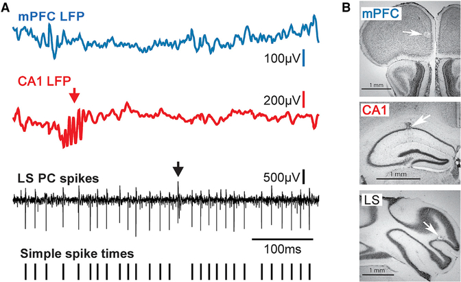
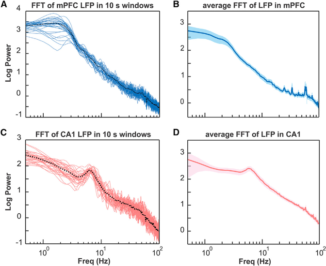
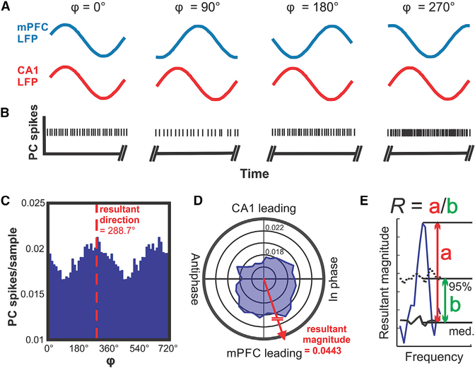
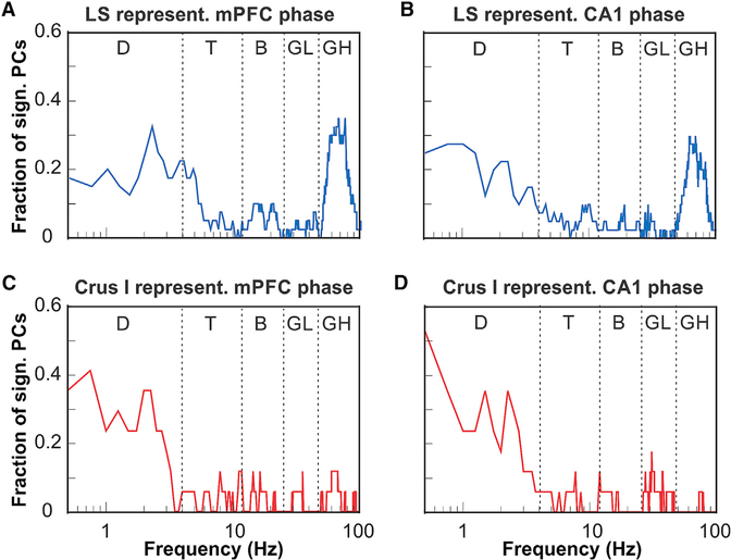
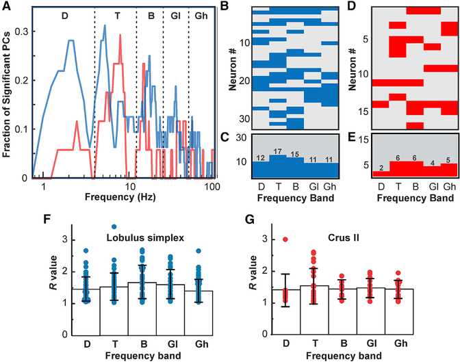
The cerebellum has long been implicated in tasks involving precise temporal control, especially in the coordination of movements. Here we asked whether the cerebellum represents temporal aspects of oscillatory neuronal activity, measured as instantaneous phase and difference between instantaneous phases of oscillations in two cerebral cortical areas involved in cognitive function. We simultaneously recorded Purkinje cell (PC) single-unit spike activity in cerebellar lobulus simplex (LS) and Crus I and local field potential (LFP) activity in the medial prefrontal cortex (mPFC) and dorsal hippocampus CA1 region (dCA1). Purkinje cells in cerebellar LS and Crus I differentially represented specific phases and phase differences of mPFC and dCA1 LFP oscillations in a frequency-specific manner, suggesting a site- and frequency-specific cerebellar representation of temporal aspects of neuronal oscillations in non-motor cerebral cortical areas. These findings suggest that cerebellar interactions with cerebral cortical areas involved in cognitive functions might involve temporal coordination of neuronal oscillations.

Keywords: cerebro-cerebellar interaction; neuronal oscillation; oscillation phase; phase difference.

Figure 1.. Raw LFP and Single-Unit Spike Signals and Anatomical Reconstructions of Recording Sites

(A) Raw LFPs recorded in the mPFC (blue trace) and CA1 (red trace), and raw single-unit PC spike activity recorded in the cerebellar LS (black trace). The arrow in the LFP recording from the CA1 region points to a sharp wave ripple event, a brief high-frequency oscillation characteristic for the hippocampus. The presence of sharp wave ripples in the LFP recordings was used for online verification of electrode tip placement within CA1. The arrow in the trace of raw PC spike activity marks the occurrence of a complex spike, which reflects input from the inferior olive. Complex spikes are characteristic for PCs and were used for online identification of PC activity. The bottom trace shows tick marks representing the time sequence of simple spikes extracted from the raw trace and used for subsequent analysis. (B) Photomicrographs of Nissl-stained sections of the mPFC, CA1, and cerebellar LS showing microlesions at recording sites (white arrows). Scale bars in all three panels are 1 mm.

Figure 2.. FFT Analysis of LFP Activity Recorded in the mPFC and Hippocampal CA1 Region at Different Times during the Recording and Averaged across Recording Time

(A) Power spectral density of LFP activity in the mPFC calculated for subsequent 10 s wide time windows (blue lines) for a 5.5 min recording session in one mouse. Dotted black line represents average FFT for the entire recording session. (B) FFT of LFP recorded in the mPFC averaged across all mice (n = 11). Shaded area represents SEM. (C) Power spectral density of LFP activity recorded in the hippocampal CA1 region calculated for subsequent 10 s wide time windows (red lines) for a 5.5 min recording session in one mouse. Dotted black line represents average FFT for the entire recording session. (D) FFT of LFP recorded in the hippocampal CA1 region averaged across all mice (n = 11). Shaded area represents SEM.

Figure 3.. Conceptual Illustration of the Data Analysis Applied to Determine the Correlation between Phase Differences of mPFC-CA1 Oscillatory LFP Activity and Those of PC Simple Spike Activity in LS

(A) Illustration of hypothetical oscillations at a specific frequency occurring simultaneously in the mPFC (blue traces) and CA1 (red traces) and displaying different phase relationships (φ) at different times. The phase relationship φ is defined as the phase difference relative to the mPFC oscillation. (B) Hypothetical PC spikes recorded simultaneously with the LFP activity in the mPFC and CA1 shown in (A). The rate modulation of this hypothetical PC shows a significant increase in spike firing when the phase difference between mPFC and CA1 oscillations reaches values around 270°. (C) Phase histogram of real PC simple spike activity. The histogram shows spike activity as a function of mPFC-CA1 phase differences at 11 Hz. The simple spike activity of the PC in this example was significantly modulated as a function of mPFC-CA1 phase difference, with a preference of 288.7°. (D) Same data as in (C) represented in polar coordinates. Vectors composed of the angular value φ and the magnitude of the spikes per sample were summated to determine the angular preference of PC activity. The resultant vector magnitude was taken to quantify the degree of modulation and tested against surrogate results for statistical significance. (E) Illustration of the quantitative evaluation of the strength of representation (R) of the mPFC-CA1 phase difference in PC spike trains. The solid blue line represents the resultant vector magnitude plotted as a function of frequency. The solid black line (med., median) and dotted black line (95%) represent the bootstrap-statistics-derived median and 95^th percentile boundary of the surrogate distribution, respectively. Resultant magnitude peak values exceeding the 95^th percentile boundary were expressed as the ratio (R) of the peak resultant magnitude value minus the surrogate median (red double arrow a) and the difference between the surrogate distribution’s 95^th percentile and the median values (green double arrow b) for the corresponding frequency.

Figure 4.. Representations of the Phase of Oscillatory LFP Activity in the mPFC and CA1 by Cerebellar PCs in Lobulus Simplex and Crus I

(A) Fraction of PCs in LS (n = 32) whose simple spike activity was significantly modulated by the oscillatory phase plotted as a function of mPFC oscillation frequency (plotted on a log-10 scale). The function shows two peaks at the delta frequency range (0.5–4 Hz) and the high gamma range (50–100 Hz). (B) As in (A) but showing fractions of LS PCs significantly modulated by the phase of oscillatory activity in CA1. (C) Fraction of PCs in Crus I (n = 17) whose simple spike activity was significantly modulated by the oscillatory phase in mPFC plotted as a function of LS oscillation frequency. The function shows a single peak at the delta frequency range (0.5–4 Hz). (D) As in (C) but showing fractions of Crus I PCs significantly modulated by the phase of oscillatory activity in CA1. D, delta; T, theta; B, beta; LG, low gamma; HG, high gamma.

Figure 5.. Individual Examples of PCs from LS and Crus I, Showing mPFC-dCA1 Phase Difference Representation in PC Simple Spike Activity

(A) Results for a representative PC recorded in LS. The blue line shows the depth of PC spike modulation, as measured by the resultant vector magnitude. Significance cutoffs represent the 95^th percentile and 99^th percentile boundaries, respectively, of the surrogate result distributions for each frequency obtained by shifting the PC spike recording in time relative to LFPs 200 times. Asterisks indicate frequencies with significant modulation (p < 0.01). (B) Pseudocolor plot shows LS PC spike density as a function of phase difference (φ) between mPFC and CA1 LFP oscillations across frequencies between 0.5 and 100 Hz. Analysis was performed within frequency bands with a 0.5–10 Hz width, in steps of 0.25 Hz. (C and D) Results for a representative PC recorded in Crus I. Plots are as in (A) and (B) but for a PC recorded in Crus I.

Figure 6.. Summary of the Representation of mPFC-dCA1 Phase Differences in PC Spike Activity and Evaluation of Representation Strength for PCs in LS and Crus I Grouped by Frequency Band

(A) Plot depicting the fraction of PCs with significantly modulated simple spike activity (p < 0.01) within each 0.25 Hz frequency step between 0.5 and 100 Hz in LS (blue graph, n = 32) and Crus I (red graph, n = 17). Modal peaks were observed within each of the conventional frequency bands: delta (D; 0.5–4 Hz), theta (T; 4–12 Hz), beta (B; 12–25 Hz), low gamma (GL; 25–45 Hz), and high gamma (GH; 45–100 Hz). (B) Pseudocolor matrix with rows representing individual PCs and columns representing frequency bands. Blue fields indicate a significant correlation between PC simple spike activity in LS and mPFC-dCA1 phase differences in each frequency band (p < 0.01). Gray fields indicate no significant correlation. (C) Histogram showing the number of PCs with significant spike-phase difference correlations within each frequency band. (D and E) Pseudocolor matrix (D) and histogram (E) are as (B) and (C), respectively, but representing results from Crus I. (F) Strength of mPFC-dCA1 phase difference representation by PCs in LS. R expresses resultant vector magnitude as the ratio of the vector length to the 95^th percentile boundary, each relative to the median surrogate value. R values were grouped by frequency band. Each dot represents the resultant vector magnitude of a PC. Bars represent the mean R for each frequency band. Error bars represent SD. (G) As in (F) but showing results for Crus I.

References

1. Bastos AM, Vezoli J, and Fries P (2015). Communication through coherence with inter-areal delays. Curr. Opin. Neurobiol 31, 173–180. - PubMed
1. Bostan AC, Dum RP, and Strick PL (2013). Cerebellar networks with the cerebral cortex and basal ganglia. Trends Cogn. Sci 17, 241–254. - PMC - PubMed
1. Braitenberg V (1961). Functional Interpretation of Cerebellar Histology. Nature 190, 539–540.
1. Braitenberg V (1967). Is the Cerebellar Cortex a Biological Clock in the Millisecond Range? Prog. Brain Res 25, 334–346. - PubMed
1. Braitenberg V, Heck D, and Sultan F (1997). The detection and generation of sequences as a key to cerebellar function: experiments and theory. Behav. Brain Sci 20, 229–245, discussion 245–277. - PubMed
Publication types
MeSH terms
LinkOut - more resources