A photometric stereo-based 3D imaging system using computer vision and deep learning for tracking plant growth

Abstract

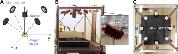
Background: Tracking and predicting the growth performance of plants in different environments is critical for predicting the impact of global climate change. Automated approaches for image capture and analysis have allowed for substantial increases in the throughput of quantitative growth trait measurements compared with manual assessments. Recent work has focused on adopting computer vision and machine learning approaches to improve the accuracy of automated plant phenotyping. Here we present PS-Plant, a low-cost and portable 3D plant phenotyping platform based on an imaging technique novel to plant phenotyping called photometric stereo (PS).

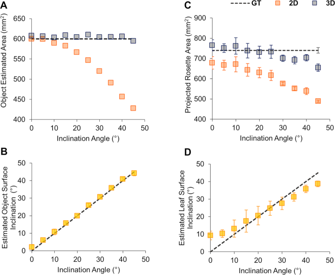
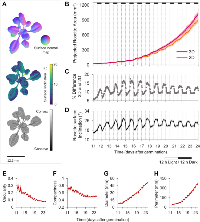
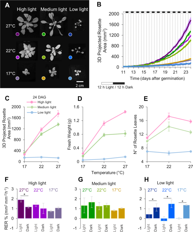
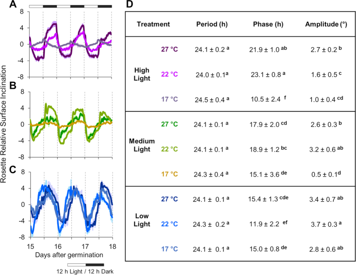
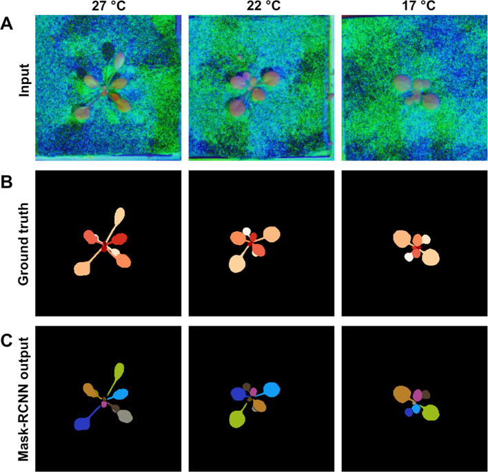
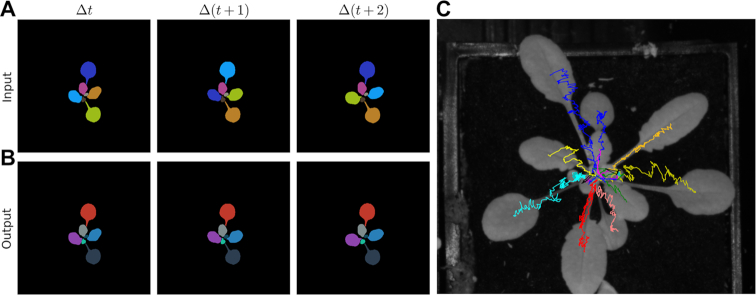
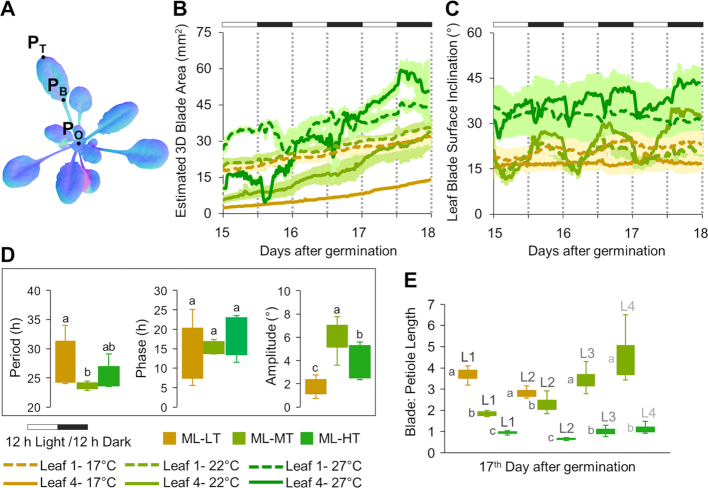
Results: We calibrated PS-Plant to track the model plant Arabidopsis thaliana throughout the day-night (diel) cycle and investigated growth architecture under a variety of conditions to illustrate the dramatic effect of the environment on plant phenotype. We developed bespoke computer vision algorithms and assessed available deep neural network architectures to automate the segmentation of rosettes and individual leaves, and extract basic and more advanced traits from PS-derived data, including the tracking of 3D plant growth and diel leaf hyponastic movement. Furthermore, we have produced the first PS training data set, which includes 221 manually annotated Arabidopsis rosettes that were used for training and data analysis (1,768 images in total). A full protocol is provided, including all software components and an additional test data set.

Conclusions: PS-Plant is a powerful new phenotyping tool for plant research that provides robust data at high temporal and spatial resolutions. The system is well-suited for small- and large-scale research and will help to accelerate bridging of the phenotype-to-genotype gap.

Keywords: Arabidopsis thaliana; leaf angle; machine learning; near-infrared LEDs; photomorphogenesis; segmentation; thermomorphogenesis.

Figure 1:

Capturing dynamic plant growth traits using photometric stereo imaging. (A) PS comprises a circular arrangement of NIR LEDs with a central camera positioned above the plant(s). Red dashed lines show the direction of light vectors. (B, C) Assembled PS-Plant system shown from side and top views. Each LED is attached to a dedicated heatsink and angled at 30° using a custom 3D-printed bracket to minimize the light distribution across the field of view. Both the camera and light sources are stationary.

Figure 2:

Evaluating the accuracy of PS-Plant with 2D and 3D data. (A, B) The estimated area and inclination angle of a flat, matte object (600 mm²) from 0° to 45° at 5° intervals. Each data point represents the average of 30 randomly selected regional patches of varying size (35–600 mm²). (C, D) The area of 3 similarly sized Arabidopsis whole rosettes (750 ± 13.5 mm²) and leaf inclination angles were estimated from 0° to 45° at 5° intervals. The dashed black lines indicate ground truth (GT) measurements. Error bars represent SD of the means.

Figure 3:

Data outputs of PS-Plant for Arabidopsis. (A) Surface normal map (top) rendered for a wild-type Arabidopsis rosette used to derive models for surface inclination (middle) and convexity (bottom). (B) Projected rosette area estimates captured for wild-type plants under standard growth conditions (22°C, 150 µmol photons m⁻² s⁻¹, 12:12 h light:dark) for 2D and 3D data from the mean ± SE values of 13 biological replicates. (C) Percentage difference between 2D and 3D estimations. (D) Estimated rosette mean inclination angles across the rosette surface. (E−H) Circularity, compactness, diameter, and perimeter estimates derived from 2D data.

Figure 4:

PS-Plant shows that Arabidopsis plants grown under different conditions show differences in growth architecture. (A) Wild-type Arabidopsis plants (24 DAG) following growth under 9 different light and temperature conditions. (B) Estimated 3D projected rosette area growth of rosettes grown under the different environments. (C–E) Estimated 3D projected area, fresh weights, and leaf count for rosettes at 24 DAG. (F–H) The average relative expansion rate (RER) during light and dark periods for each growth condition (calculated from 15–18 DAG with a 4-hr sliding window). Values represent the mean ± SE values of ≥3 biological replicates. Asterisks indicate significant differences between light and dark values for each condition based on Student's t-test (P < 0.05). The colour legends in A are applicable to B, and F–H.

Figure 5:

Arabidopsis plants grown under different conditions show differences in circadian movement. (A-C) The relative rosette surface inclination (i.e., rosette surface inclination following baseline detrending and alignment to the mean) for plants grown in high, medium, and low light from 15 to 18 DAG (see Supplementary Figure S3 for full data sets). (D) Period, phase, and amplitude calculated by the MFourFit method [87] using data from 11–24 DAG. Values are the mean ± SD of measurements made on ≥3 biological replicates. Values within each column followed by different letters are significantly different from each other and values followed by the same letter are not (P < 0.05) as determined by ANOVA followed by Tukey's HSD tests.

Figure 6:

Automated segmentation of individual Arabidopsis leaves using PS-Plant data. Examples are shown based on the Mask R-CNN architecture for plants grown in ML at 3 different temperatures. (A) Composite input images are composed of surface normals in x, y directions and albedo data. (B) Manually labelled images (ground truth) used for training. (C) Mask R-CNN output images showing automated leaf segmentation. For ground truth images and Mask R-CNN outputs each leaf was assigned a unique arbitrary colour.

Figure 7:

Automated tracking of leaf labels from segmented Arabidopsis rosettes. (A) Three consecutive frames for labelled leaves produced using the trained Mask R-CNN architecture (as in Fig. 6). (B) Tracked leaves retained the same colour after application of label tracking (see Rich Media 4). The particle filter allowed calibration of a variety of parameters, including span (the velocity of "span + 1" recent frames), search radius (the farthest distance [in pixels] an object may travel between frames), frame memory (the maximum number of frames a seen/tracked object that is absent will be remembered), and filter (the minimum number of frames in which an object must be seen/tracked to be included). The following particle filter settings produced the best results: span (10), search radius (30), frame memory (3), and filter (100). (C) Example of leaf tracking using leaf centroid locations. Each coloured line represents the movement of the centroid location of an individual leaf from 11 to 24 DAG.

Figure 8:

Analyses of growth and movement for individual leaves. (A) Key landmarks for leaf analysis: rosette origin (P_O), leaf base/leaf blade and petiole intersection point (P_B), and leaf tip (P_T). Data are shown from plants grown in ML at 3 different temperatures (17°C [LT], 22°C [MT], or 27°C [HT]). (B, C) Leaf blade area and mean surface inclination of a maturing leaf (leaf 1) and an immature leaf (leaf 4) from 15 to 18 DAG. Error bars represent the mean ± SE of 3 separate leaves. (D) Period, phase, and amplitude values of the leaf blade from immature leaves (leaves 3 and 4; n = 6 leaves). Letters above the error bars indicate significant differences within each data type (P < 0.05) as determined by ANOVA followed by Tukey's HSD tests. Data sets with the same letter are not significantly different. (E) The ratio of leaf blade to petiole length for leaves 1–4 (L1–L4). Values represent the mean ratio over 24 h (17–18 DAG) for 3 separate leaves. Letters indicate significant differences (P < 0.05) within each leaf data set for different temperatures (i.e., L1, L2, L3, and L4).

References

-
- Meinke H. Agricultural impacts: Europe's diminishing bread basket. Nat Clim Chang. 2014;4:541–2.
- Long SP, Marshall-Colon A, Zhu XG. Meeting the global food demand of the future by engineering crop photosynthesis and yield potential. Cell. 2015;161:56–66. - PubMed
Publication types
MeSH terms
Grants and funding
LinkOut - more resources
Full Text Sources
Molecular Biology Databases
Miscellaneous