Parameter estimation and identifiability in a neural population model for electro-cortical activity

Abstract

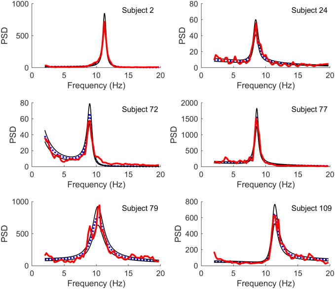
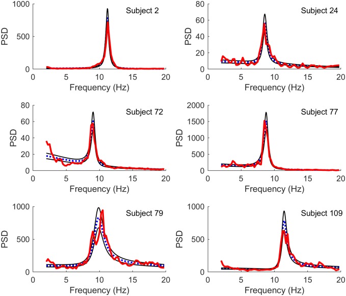
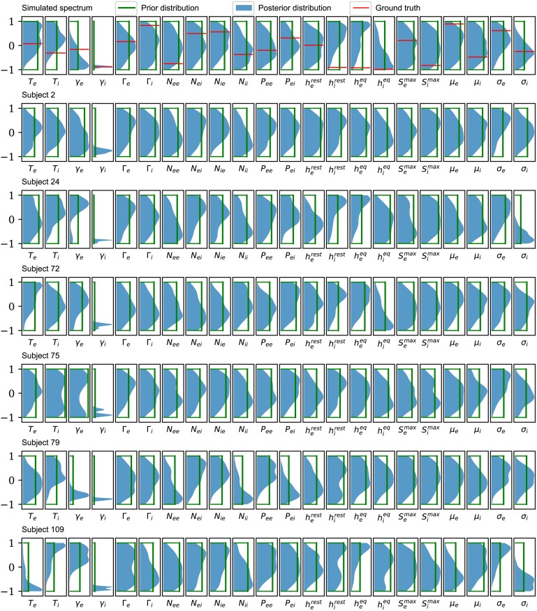
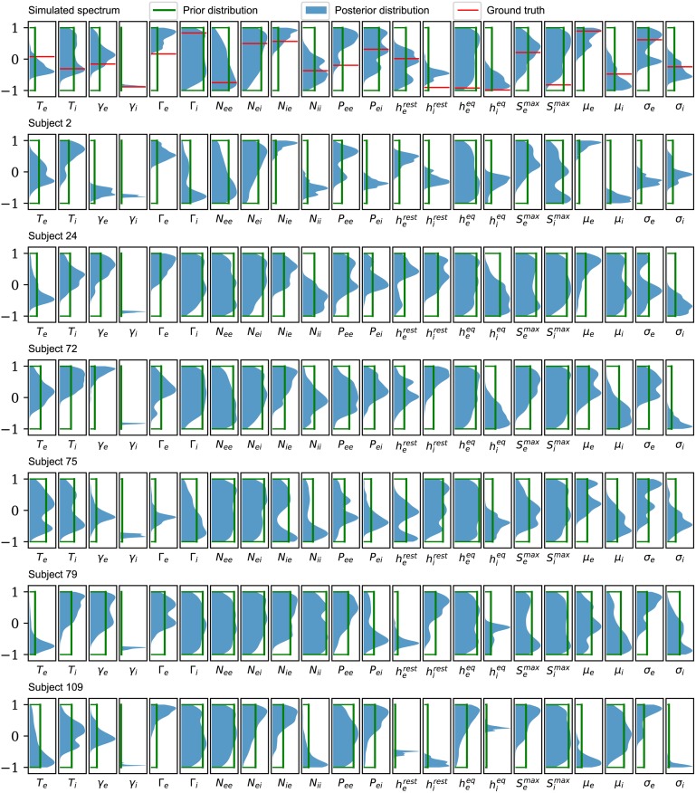
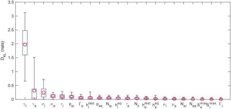
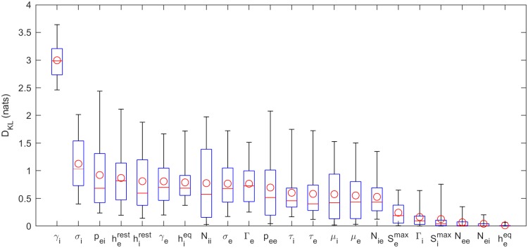
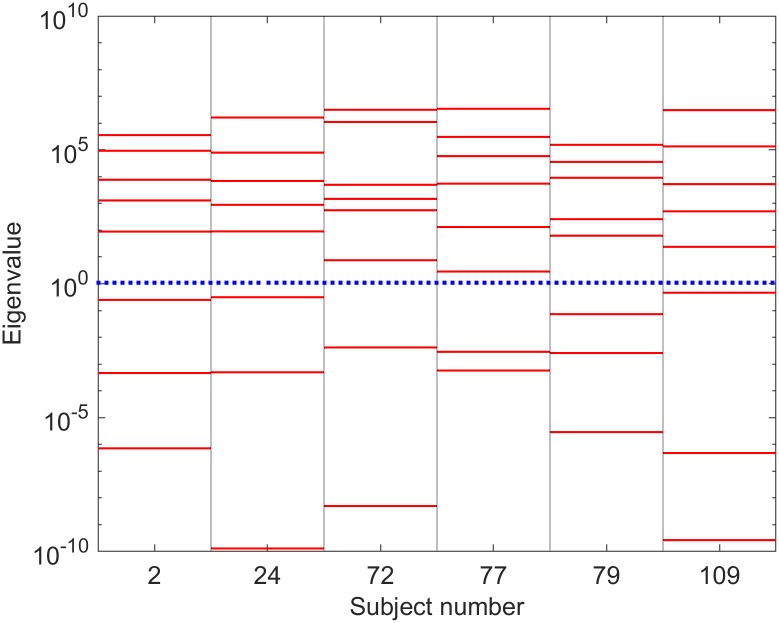
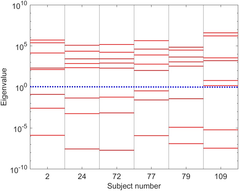
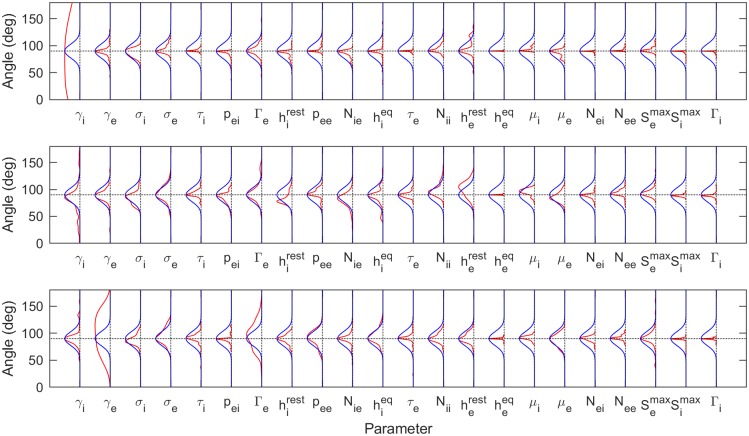
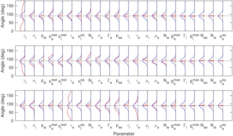
Electroencephalography (EEG) provides a non-invasive measure of brain electrical activity. Neural population models, where large numbers of interacting neurons are considered collectively as a macroscopic system, have long been used to understand features in EEG signals. By tuning dozens of input parameters describing the excitatory and inhibitory neuron populations, these models can reproduce prominent features of the EEG such as the alpha-rhythm. However, the inverse problem, of directly estimating the parameters from fits to EEG data, remains unsolved. Solving this multi-parameter non-linear fitting problem will potentially provide a real-time method for characterizing average neuronal properties in human subjects. Here we perform unbiased fits of a 22-parameter neural population model to EEG data from 82 individuals, using both particle swarm optimization and Markov chain Monte Carlo sampling. We estimate how much is learned about individual parameters by computing Kullback-Leibler divergences between posterior and prior distributions for each parameter. Results indicate that only a single parameter, that determining the dynamics of inhibitory synaptic activity, is directly identifiable, while other parameters have large, though correlated, uncertainties. We show that the eigenvalues of the Fisher information matrix are roughly uniformly spaced over a log scale, indicating that the model is sloppy, like many of the regulatory network models in systems biology. These eigenvalues indicate that the system can be modeled with a low effective dimensionality, with inhibitory synaptic activity being prominent in driving system behavior.

Fig 1. Best fits using least squares.

Comparison of model spectra (blue dotted line) fit to experimental spectra (red thick line) by least squares (LS) minimization using particle swarm optimization, for a select set of subjects. Also shown are the 16% and 84% quantiles based on the gamma distribution for the fitted spectra (thin black lines). The subjects have been selected to show the range of spectra included in the full data set. A comparison of the experimental time series with representative samples of modelled time series for the same subjects is included in S1 Fig.

Fig 2. Best fits using maximum likelihood.

Comparison of model spectra (blue dotted line) fit to experimental spectra (red thick line) by maximum likelihood (ML) estimation using MCMC. Also shown are the 16% and 84% quantiles (thin black lines). The subjects are the same as in Fig 1. It should be noted that LS and ML fits are expected to differ in this case, since the LS fits are more sensitive to deviations in the unweighted spectral power (typically in regions with larger power) whereas the ML fits are more sensitive to deviations in regions where the variance of spectral power is small (typically in regions of lower spectral power).

Fig 3. Posterior distributions based on PSO sampling.

Comparison of the posterior (solid color) and prior marginal (green line) distributions for the selected subjects used in Figs 1 and 2. For the simulated spectrum (first row), the distributions of the parameters are presented against the ground truths for the corresponding parameters (red line). The distributions are based on kernel density estimates from the best 100 of 1000 randomly seeded particle swarm optimizations for each subject. The seeds are uniformly distributed over the allowed parameter ranges. The major result is that, across the full set of 82 subjects, only the parameter γ_i is significantly constrained. All other parameters have nearly the same uncertainties as the prior.

Fig 4. Posterior distributions based on MCMC sampling.

Comparison of the posterior marginal distributions (solid color) with the prior marginal distributions (green line) for the selected subjects used in Figs 1 and 2. For the simulated spectrum (first row), the distributions of the parameters are presented against the ground truths for the corresponding parameters (red line). Each distribution is based on a kernel density estimate from 1000 samples (sub-sampled from 10⁶MCMC samples). Consistent with the conclusions from PSO sampling, only γ_i is consistently constrained by the data when viewed across all subjects.

Fig 5. KLDs based on PSO samples.

Kullback-Leibler divergences of marginal posterior parameter distributions calculated relative to uniform prior distributions. The posteriors are based on the best 100 of 1000 randomly seeded runs of particle swarm optimization (see Fig 3). The boxes represent the 25% and 75% quartiles; the whiskers represent the 5% and 95% quantiles; the red lines show the median KLDs and the circles the mean KLDs over the full set of 82 subjects.

Fig 6. KLDs based on MCMC samples.

Kullback-Leibler divergences of marginal posterior parameter distributions (see Fig 4). Here kernel density estimates based on 1000 MCMC samples of the posterior parameter distribution are used.

Fig 7. FIM eigenspectra based on LS best fits.

Leading eigenvalues of the FIM for selected subjects. The FIM is numerically calculated using dimensionless increments at the parameters corresponding to a least squares fit to the experimental spectrum. Of the 22 possible eigenvalues, roughly 7 correspond to zero, at least to the numerical accuracy of the eigenvalue estimation routine. Typically 7 of the remaining 15 are too small (relative to the largest eigenvalue) to be reliably calculated using the Matlab^™ eig command. The roughly uniform distribution of the eigenvalues on a log scale is a characteristic of a sloppy model. The blue dotted line delineates the separation of identifiable (above the dotted line) from unidentifiable (below the dotted line) regimes [43]. Thus ∼5 parameter combinations are usually identifiable, suggesting that the 22-parameter model can be described using 5 or 6 effective parameters. A comprehensive plot of the FIM eigenspectra for all subjects is included in S2 Fig; the spectra observed above are typical of those seen across the full set of subjects.

Fig 8. FIM eigenspectra based on ML best fits.

This is similar to Fig 7, except here the FIM is calculated around the best fit found from maximum likelihood optimization for each subject’s spectrum.

Fig 9. Contributions to the eigenvectors corresponding to 1^st, 2^nd and 3^rd eigenvalues based on LS best fits.

Alignment of the leading eigenvectors relative to each parameter. 0° and 180° represent perfect alignment (maximum contribution) whereas 90° represents orthogonality (no contribution). To compare the 82 subjects, results are presented as angular distributions (red lines). The first row is for the largest eigenvalue, the second row for the second-large eigenvalue, etc. The blue lines show the expected angular distributions for a randomly pointed vector in the 22-dimensional parameter space, illustrating how these are most likely to be orthogonal to any parameter direction. The angles are the inverse cosines of the direction cosines of the vectors. The distributions indicate that the parameters γ_i and (to a lesser extent) γ_e may play significant roles in determining the spectral form in their own right. The remaining parameters appear largely in complicated combinations.

Fig 10. Components of eigenvectors corresponding to 1^st, 2^nd and 3^rd eigenvalues based on ML best fits.

As for Fig 9, but using the ML best fits, again showing the significant roles played by the parameters γ_i and γ_e.

Fig 11. The model as a simple feedback system.

The transfer function of the system $T(s)=\frac{H_1(s)}{1+H_1(s)H_2(s)}$ where both H₁(s) and H₁(s) are third order filters.

References

1. Kropotov JD. Chapter 2—Alpha Rhythms In: Kropotov JD, editor. Quantitative EEG, Event-Related Potentials and Neurotherapy. San Diego: Academic Press; 2009. p. 29–58. Available from: http://www.sciencedirect.com/science/article/pii/B9780123745125000025.
1. Aminoff MJ. Chapter 3—Electroencephalography: General Principles and Clinical Applications In: Aminoff MJ, editor. Aminoff’s Electrodiagnosis in Clinical Neurology (Sixth Edition) sixth edition ed. London: W.B. Saunders; 2012. p. 37–84. Available from: http://www.sciencedirect.com/science/article/pii/B9781455703081000030.
1. Berger H. Über das elektrenkephalogramm des menschen. Archiv für psychiatrie und nervenkrankheiten. 1929;87(1):527–570. 10.1007/BF01797193 - DOI
1. Berger H. On the electroencephalogram of man. Third Report 1931; Twelfth Report 1937. Translated by Pierre Gloor. Electroencephalogr Clin Neurophysiol. 1931;28(suppl):113–167.
1. Lozano-Soldevilla D. On the Physiological Modulation and Potential Mechanisms Underlying Parieto-Occipital Alpha Oscillations. Front Comput Neurosci. 2018;12:23 10.3389/fncom.2018.00023 - DOI - PMC - PubMed
Publication types