The Heterogeneity Problem: Approaches to Identify Psychiatric Subtypes

Abstract

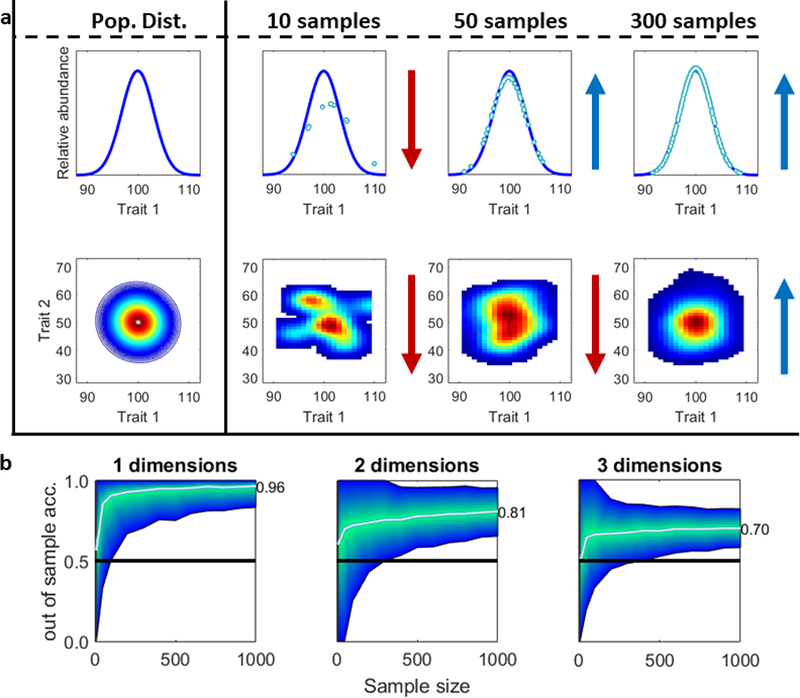
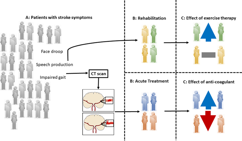
The imprecise nature of psychiatric nosology restricts progress towards characterizing and treating mental health disorders. One issue is the 'heterogeneity problem': different causal mechanisms may relate to the same disorder, and multiple outcomes of interest can occur within one individual. Our review tackles this heterogeneity problem, providing considerations, concepts, and approaches for investigators examining human cognition and mental health. We highlight the difficulty of pure dimensional approaches due to 'the curse of dimensionality'. Computationally, we consider supervised and unsupervised statistical approaches to identify putative subtypes within a population. However, we emphasize that subtype identification should be linked to a particular outcome or question. We conclude with novel hybrid approaches that can identify subtypes tied to outcomes, and may help advance precision diagnostic and treatment tools.

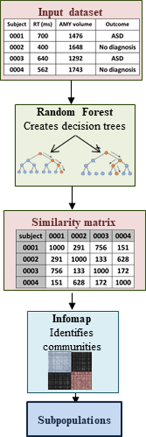
Keywords: functional random forest; heterogeneity; machine learning; mental health; surrogate variable analysis.

Figure 1. Data simulations showing the ‘curse of dimensionality.’

[69] Examining mental health disorders or cognitive behaviors considering only 1-continuous distribution using a purely dimensional framework (i.e., without considering subtypes) is challenging. (A). Data were simulated for correlated traits from Gaussian distributions (i.e., “Pop Dist.”). Trait 1 measure (x-axis) and frequency (y-axis) is plotted in the top row. The two dimensional density for traits 1 (x-axis) and 2 (y-axis) are plotted in the bottom row. The leftmost panels show the population distributions for the traits. From there we randomly sample “subjects” from the distribution. As shown, the number of “subjects” needed to approximate the distribution rises from 10 samples to 300 samples as the number of dimensions (i.e. traits) increases from one (top) to two (bottom). Good (blue arrows) and poor (red arrows) population fits are indicated. (B) Outlier detection was conducted [124] for one (left), two (middle), and three dimensions (right). Data were sampled from a multivariate normal distribution (means = 0, s.d = 1), to satisfy the method used. Thresholds for true outliers were determined from a large sample (N=10,000). To test outlier accuracy, smaller samples (N= 10 to N = 1000) were pseudo-randomly generated 1000 times and true outliers identified using the known threshold. Correctly identified outliers were calculated as the percentage of identified true outliers divided by the total true outliers. As shown, the accuracy of identifying true outliers decreases as the number of dimensions is examined. Code to reproduce these plots can be found at (http://github.com/dcan-labs).

Figure 2. Key Figure. U.S. populations maps reveal profound heterogeneity.

Several valid and important ways that a population might be subdivided are shown here. Each one of these subdivisions are useful for different types of questions and analogous to parsing clinical and cognitive heterogeneity. (A) Subtypes across the United States based on dialect preferences for ‘soda’, ‘pop’, or ‘coke’. Counties are colored by the most commonly used term. Language preferences were derived from Alan McConchie’s “pop vs. soda” survey (http://popvsoda.com/). Three subtypes were identified by the survey. East/West coast form one subtype that uses “soda”. Southeast people use “coke”, perhaps reflecting that Coca-Cola is headquartered in Atlanta. The northern/upper Midwest uses “pop”. (B) Subtypes across the United States based on the 2016 presidential election. Data were from Tony McGovern’s repository (https://github.com/tonmcg/County_Level_Election_Results_12–16). Difference between Democrat (blue) and Republican (red) voting percentages are plotted by county. Two subtypes can be seen from voting preferences. “Urban” counties centered around cities typically voted more Democrat. “Rural” counties typically voted more Republican. (C) Subtypes across the United States using data from the National Center for Health Statistics (https://www.cdc.gov/nchs/data_access/vitalstatsonline.htm). Stroke mortality rates for adults aged 35 years or older are plotted by county. One cluster can be seen in the eastern states, excluding the Northeast and tip of Florida, and another can be seen on the West coast. Code to reproduce these maps (http://github.com/dcan-labs) was written in R with the ggplot2[125] and maps[126] package. Color bar was resized and relabeled for visibility in this figure.

Figure 3. Stroke example shows the heterogeneity problem.

(A) Unlabeled cases (grey) first present with behavioral symptoms like face droop, impaired speech production, or impaired gait. Cases then undergo a CT scan to determine the cause of the stroke. (B) Four cases are labeled based on clinician identified outcomes such as the use of the anti-coagulant, warfarin. Patient are ‘sub-grouped’ into ischemic (blue) or hemorrhagic (red) stroke groups as determined from CT scans. (C) Effect of warfarin treatment on outcome. The effect of anti-coagulants during acute treatment, where anti-coagulants may harm cases with hemorrhagic stroke but benefit cases with ischemic stroke. In this instance, being able to sub-group individuals outside of signs and symptoms is critical for treatment. (D) The same exact cases as in (B); however, cases are now grouped by impaired gait (green) or speech (yellow) as determined from stroke symptoms. (E) The effect of exercise therapy during rehabilitation, which benefits impaired gait but not impaired speech, is also dependent on the distinct sub-grouping (D). Populations, such as stroke populations can be sub-divided into subgroups in many different ways. Which possibility is the most important depends in large part on the question of interest.

Figure 4. FRF identifies subtypes relevant to the question of interest.

The FRF attempts to identify subtypes tied to a specific outcome or measure. Input datasets (top red panel) are input into a RF algorithm. Input data can comprise measures with any distributions, and can even be categorical. Outcomes may be continuous or categorical variables. Input data are split into testing and training datasets, preferably by 5- or 10-fold cross validation (see Box 1). The RF[90] (green panel) comprises an ensemble of decision trees. Per tree, a subset of the training data is bootstrap resampled and used to construct the decision tree. Per branch, a random subset of measures is selected. The selected measure that best splits the data according to the outcome forms the rule for the given branch. Trees stop growing when data are sufficiently divided into appropriate bins, called “terminal nodes”, reflecting the same or similar outcome measure. Testing data are evaluated for each tree, which votes on the data, and the predicted outcome is calculated by averaging the votes. Individuals may take different paths (red lines) that predict the same outcome. By counting these paths, one can form a similarity matrix (lower red panel) for input or independent datasets, and the matrix reflects the total number of times participants traverse the same paths through the forest. This matrix is recast as a graph and input into an Infomap algorithm[92] (light blue panel), which uses a random walker to identify subtypes (bottom panel).

Figure 5. Functional connectivity patterns vary by FRF identified subtype.

This figure was modified from [59] where the FRF was applied to behavioral data. Sufficient fcMRI data was obtained for three ASD subgroups (ASD SG1, ASD SG2, ASD SG3) and one typical subgroup ( CON SG1 - see legend). A chi-squared analysis was performed, using systems identified by Gordon et al[127] to determine within or between network systems that were differentially atypical amongst these groups (see brain inset). Briefly, the chi-squared analysis tests whether the number of significantly varying connections within or between two communities are greater than what would be observed by chance. Here, the analysis reveals intra- and inter-system effects of subgroup. Seven effects were found that showed varying effects relative to the control group with respect to the ASD subgroups. Four are displayed here. (AUD-CIP) ASD subgroup 1 shows increased connectivity between auditory (AUD) and Cingulo-Parietal (CIP) systems. (CIO-DEF) ASD subgroups 2 and 3 show increased connectivity between Cingulo-opercular (CiO) and default (DEF) systems. (DEF-DEF) All three ASD subgroups show decreased connectivity within the default (DEF) system). (DEF-SMH) ASD subgroup 3 shows elevated connectivity between default (DEF) and somatomotor-hand (SMH) systems, while ASD subgroup 2 shows decreased connectivity. Taken together, these findings highlight differential connectivity patterns that do not reflect simple severity, even though the subgroups were identified from behavioral data.

Figure 6. FRF can identify subtypes from longitudinal trajectories.

Input dataset (center red panel) comprise at least 4 time points per case. Preferably, the first and last time point occur at the same time across the cases. B-spline basis functions[123] are fit to each case’s time series. (hybrid red panel) Per case, parameters are extracted from the fit functions and entered into the FRF (see: Figure 4). Model-based subtypes identified through this approach can be tied to a question. Subtypes can also be identified through an unsupervised approach (unsupervised blue panel). First, a correlation matrix is produce by calculating the correlation between each case’s predicted trajectory. The correlation matrix is then entered into Infomap, which identifies the correlation based subtypes.

References

1. Kendler KS (2009) An historical framework for psychiatric nosology. Psychol. Med 39, 1935–1941 - PMC - PubMed
1. Nigg JT (2006) Temperament and developmental psychopathology. J. Child Psychol. Psychiatry 47, 395–422 - PubMed
1. Mason D and Hsin H (2018) ‘A more perfect arrangement of plants’: the botanical model in psychiatric nosology, 1676 to the present day. Hist. Psychiatry 29, 131–146 - PubMed
1. Organization, W.H. and others (1996) Multiaxial classification of child and adolescent psychiatric disorders: the ICD-10 classification of mental and behavioural disorders in children and adolescents, Cambridge Univ Pr.
1. Robins LN et al. (1981) National Institute of Mental Health Diagnostic Interview Schedule: Its history, characteristics, and validity. Arch Gen Psychiatry 38, 381–389 - PubMed
Publication types